Stem Cell

A human neural crest model reveals the developmental impact of neuroblastoma-associated chromosomal aberrations – Nature Communications

Time Stamp: May 2, 2024 8:00 PM
Source Node: 586436

Human embryonic stem cell (hESC) cell culture and differentiation

Cell lines and cell culture

We employed H7 (https://hpscreg.eu/cell-line/WAe007-A) and H9 (https://hpscreg.eu/cell-line/WAe009-A) hESCs as karyotypically normal, female WT controls³⁸. Use of human embryonic cells has been approved by the Human Embryonic Stem Cell UK Steering Committee (SCSC23-29). Their isogenic chr17q counterparts carry a gain in chromosome 17q (region q27q11) via an unbalanced translocation with chromosome 6 (H7) or a gain of 17q via an unbalanced translocation with chromosome 21 with breakpoints at 17q21 and 21p11.2 (H9)^50,101. The chr17q1q hESC lines were clonally derived, after their spontaneous emergence following the genetic modification of chr17q hESCs. The H7 chr17q1q-MYCN hESC line was generated by introducing a TetOn-PiggyBac plasmid (PB-TRE3G-MYCN, plasmid#104542, Addgene) carrying the wild-type version of the MYCN gene¹⁰² while the H9 chr17q1q-MYCN and H7 WT-MYCN and 17q-MYCN hESC lines were produced using a Tet-On “all-in-one” inducible expression cassette containing the TRE3G promoter driving the expression of MYCN with a 2A peptide-linked fluorescent reporter (mScarlet) and a pCAG promoter-driven rtTA3G transactivator^103,104. Plasmids were introduced via nucleofection using either the Neon NxT Electroporation System (Thermo Fisher Scientific) or the Lonza 4D-Nucleofector System. In the case of the latter, the Amaxa 4D-Nucleofector Basic Protocol for Human Stem Cells was employed with the following modification: 2 × 10⁶ cells were transfected with 2 µg plasmid in 100 µl Nucleocuvettes. All cell lines were tested regularly for mycoplasma and expression of pluripotency markers. Karyotypic analysis was carried out using G-banding (number of cells examined = 20–30). A rapid quantitative PCR (qPCR) assay was also regularly employed to detect the emergence of common CNAs such as chr17q and 1q gains in our hESC lines¹⁰⁵. hESCs were cultured routinely in feeder-free conditions at 37 °C and 5% CO₂ in E8 media¹⁰⁶ complemented with GlutaMax (Cat# 35050061, Thermo Fisher Scientific) on Vitronectin (Cat# A14700, Thermo Fisher Scientific) or on Geltrex LDEV-Free Reduced Growth Factor Basement Membrane Matrix (Cat# A1413202, Thermo Fisher Scientific) as an attachment substrate. All hESC lines described in this manuscript are available upon request and completion of a Material Transfer Agreement.

Differentiation toward trunk neural crest

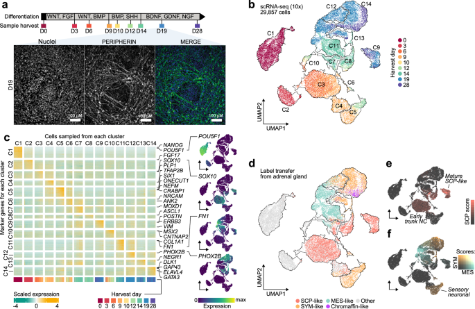
hESC differentiation toward trunk NC and its derivatives was performed using our established protocols^35,36. Briefly, hESCs were harvested using StemPro Accutase Cell Dissociation Reagent (Cat# A1110501, Thermo Fisher Scientific) and plated at 60,000 cells/cm² in N2B27 medium supplemented with 20 ng/ml of FGF2 (Cat# 233-FB/CF, R&D) and 4 μM of CHIR 99021 (Cat# 4423, Tocris) and 10 μM of Rock Inhibitor (Y-27632) (Cat# A11001, Generon) in a volume of 300 µl/cm². The N2B27 medium consisted of 50:50 DMEM F12 Merck Life Science/Neurobasal medium (Gibco) and 1x N2 supplement (Cat# 17502048, Invitrogen), 1x B27 (Cat#17504044, Invitrogen), 1x GlutaMAX (Cat# 35050061, Thermo Fisher Scientific), 1x MEM Non-essential amino acids (NEAA; Cat#11140050, Thermo Fisher Scientific), 50 μM 2-Mercaptoethanol (Cat# 31350010, Thermo Fisher Scientific). After 24 h, media was refreshed removing the Rock Inhibitor and cells were cultured for a further 2 days in FGF2/CHIR to generate NMPs (300 µl/cm²). NMPs at D3 were then re-plated at 50,000 cells/cm² (H7) or 40,000 cells/cm² (H9) in neural crest inducing medium consisting of DMEM/F12, 1x N2 supplement, 1x GlutaMAX, 1x MEM NEAA, the TGF-beta/Activin/Nodal inhibitor SB-431542 (2 μM, Cat# 1614, Tocris), CHIR99021 (1 μM, Cat# 4423, Tocris), BMP4 (15 ng/ml, Cat# PHC9534, Thermo Fisher Scientific), the BMP type-I receptor inhibitor DMH-1 (1 μM, Cat# 4126, Tocris), 10 μM of Rock Inhibitor (Y-27632) on Geltrex LDEV-Free Reduced Growth Factor Basement Membrane Matrix (Cat# A1413202, Thermo Fisher Scientific) in a volume of 300 µl/cm². 48 h later (D5), media was replaced removing the Rock Inhibitor. Media was refreshed at D7 and D8 increasing volume to 500 µl/cm². On D5, the expression of MYCN was induced by supplementing the neural crest media with 100 ng/ml (H7-17q1q-MYCN), 200 ng/ml (H7 WT-MYCN, 17q-MYCN), or 1000 ng/ml (H9-derived lines) of Doxycycline (Cat# D3447, Merck). On D9, cells were re-plated at 150,000–250,000 cells/cm² in plates coated with Geltrex (Thermo Fisher Scientific) in the presence of medium containing BrainPhys (Cat# 05790, Stem Cell Technologies), 1x B27 supplement (Cat# 17504044, Invitrogen), 1x N2 supplement (Cat# 17502048, Invitrogen), 1x MEM NEAA (Cat# 11140050, Thermo Fisher Scientific) and 1x Glutamax (Cat# 35050061, Thermo Fisher Scientific), BMP4 (50 ng/ml, Cat# PHC9534, Thermo Fisher Scientific), recombinant SHH (C24II) (50 ng/ml, Cat# 1845-SH-025, R and D) and purmorphamine (1.5 µM, Cat# SML0868, Sigma) and cultured for 5 days (=D14 of differentiation) in a volume of 250 µl/cm². Media was refreshed daily. For further sympathetic neuron differentiation, D14 cells were switched into a medium containing BrainPhys neuronal medium (Stem Cell Technologies), 1x B27 supplement (Invitrogen), 1x N2 supplement (Invitrogen), 1x NEAA (Thermo Fisher Scientific) and 1x Glutamax (Thermo Fisher Scientific), NGF (10 ng/ml, Cat#450-01 Peprotech), BDNF (10 ng/ml, Cat# 450-02, Peprotech) and GDNF (10 ng/ml, Cat# 450-10, Peprotech) for a further 5–14 days (volume of 300 µl/cm² changing media every other day). Volume was increased up to 500 µl/cm², depending on cell density, after day 17 of differentiation.

Immunostaining

Cells were fixed using 4% PFA (P6148, Sigma-Aldrich) at room temperature for 10 min, then washed twice with PBS (without Ca²⁺, Mg²⁺) to remove any traces of PFA and permeabilised using a PBS supplemented with 10% FCS, 0.1% BSA and 0.5% Triton X-100 for 10 min. Cells were then incubated in blocking buffer (PBS supplemented with 10% FCS and 0.1% BSA) for 1 h at RT or overnight at 4 °C. Primary and secondary antibodies were diluted in the blocking buffer; the former were left overnight at 4 °C and the latter for 2 h at 4 °C on an orbital shaker. Samples were washed twice with blocking buffer between the primary and secondary antibodies. Hoechst 33342 (H3570, Invitrogen) was added at a ratio of 1:1000 to the secondary antibodies’ mixture to label nuclei in the cells. We used the following primary antibodies SOX10 (D5V9L) (Cell Signalling, 89356S, 1:500); HOXC9 (Abcam, Ab50839,1:50); MYCN (Santa Cruz, SC-53993, 1:100); PHOX2B (Santa Cruz, SC-376997, 1:100); MASH1 (ASCL1) (Abcam, Ab211327, 1:100); Ki67 (Abcam, Ab238020, 1:100); PERIPHERIN (Sigma-Aldrich, AB1530, 1:400); Cleaved Caspase 3 (Asp175) (Cell Signalling, 9661S, 1:400), yH2AX (Cell Signalling, S139/9718S, 1:400). Secondary antibodies: Goat anti-Mouse Affinipure IgG+IgM (H + L) AlexaFluor 647 (Stratech (Jackson ImmunoResearch) 115-605-044-JIR, Polyclonal 1:500); Donkey anti-Rabbit IgG (H + L) Alexa Fluor 488 (Invitrogen, A-21206, 1:1000).

Intracellular flow cytometry staining

Cells were detached and resuspended as single cells using StemPro Accutase Cell Dissociation Reagent (Cat# A1110501, Thermo Fisher Scientific) and then counted. Next, 10 million cells/ml were resuspended in 4% PFA at room temperature for 10 min. Then cells were washed once with PBS (without Ca²⁺, Mg²⁺) and pelleted at 200 g. Cells were resuspended in PBS at 10 million/ml and used for antibody staining. Permeabilisation buffer (0.5% Triton X-100 in PBS with 10% FCS and 0.1% BSA) was added to each sample, followed by incubation at room temperature for 10 min. Samples were then washed once with staining buffer (PBS with 10% FCS and 0.1% BSA) and pelleted at 200 g. Then samples were resuspended in staining buffer containing pre-diluted primary antibodies: SOX10 (D5V9L) (1:500; 89356S, Cell Signalling); HOXC9 (1:50; Ab50839, Abcam); cleaved Caspase 3 (Asp175) (Cell Signalling, 9661S, 1:400). The samples were left at 4 °C on an orbital shaker overnight. Then, the primary antibodies were removed, and samples were washed two times with staining buffer. After washing, staining buffer with pre-diluted secondary antibody was added to the samples and incubated at 4 °C for 2 h. The secondary antibodies used were Goat anti-Mouse Affinipure IgG+IgM (H + L) AlexaFluor 647 (Stratech (Jackson ImmunoResearch) 115-605-044-JIR, Polyclonal 1:500); Donkey anti-Rabbit IgG (H + L) Alexa Fluor 488 (Invitrogen, A-21206, 1:1000). Finally, samples were washed once with staining buffer, resuspended in staining buffer and analysed using a BD FACSJazz or a CytoFLEX (Beckman Coulter) flow cytometer. A secondary antibody-only sample was used as a control to set the gating.

Cell cycle analysis

The 5-ethynyl-2´-deoxyuridine (EdU) assay was performed following the manufacturer’s instructions (Thermo Fisher Scientific, C10633 Alexa Fluor 488). We used 10 μM of Edu for a 2-h incubation. Cells were analysed in the flow cytometer (BD FACSJazz) using the 405 nm laser to detect the Hoechst/DAPI staining and 488 nm to detect the EdU staining.

Low-density plating

Day 9 trunk NC cells derived from hESCs as described above were harvested and plated at a density of 500 cells/cm² in plates pre-coated with Geltrex LDEV-Free Reduced Growth Factor Basement Membrane Matrix (Cat# A1413202, Thermo Fisher Scientific) in the presence of DMEM/F12 (Sigma-Aldrich), 1x N2 supplement, 1x GlutaMAX, 1x MEM NEAA, the TGF-beta/Activin/Nodal inhibitor SB-431542 (2 μM, Tocris), CHIR99021 (1 μM, Tocris), BMP4 (15 ng/ml, Thermo Fisher Scientific), the BMP type-I receptor inhibitor DMH-1 (1 μM, Tocris) and ROCK inhibitor Y-27632 2HCl (10 μM) (300 µl/cm²). The culture medium was replaced the following day with medium containing BrainPhys (Stem Cell Technologies), 1x B27 supplement (Invitrogen), 1x N2 supplement (Invitrogen), 1x NEAA (Thermo Fisher Scientific) and 1x Glutamax (Thermo Fisher Scientific), BMP4 (50 ng/ml, Thermo Fisher Scientific), recombinant SHH (C24II) (50 ng/ml, R and D) and Purmorphamine (1.5 µM, Sigma) (250 µl/cm²). Plates were then incubated at 37 °C at 5% CO₂. The media was refreshed every 48 h. After 5 days of culture, cells were fixed (PFA 4%/10 min) and stained with Hoechst 33342 (Cat# H3570, Invitrogen) for 5 min. Colonies were detected using an InCell Analyser 2200 (GE Healthcare) at a 4X magnification. Images were processed using Cell Profiler.

DNA damage analysis

DNA damage was measured by assessing the phosphorylation state of the histone H2AX on the SerCells were fixed and immunostained using the anti-yH2AX as described above at different time points. Stained cells were imaged using the InCell Analyser 2200 (GE Healthcare) at 40X magnification. Image analysis was performed using a pipeline in CellProfiler that allowed us to detect the number of foci of yH2AX antibody per nuclei.

Quantitative real-time PCR

RNA extractions were performed using the total RNA purification kit (Norgen Biotek, 17200) according to the manufacturer’s instructions. cDNA synthesis was performed using the High-Capacity cDNA Reverse Transcription kit (ThermoFisher, 4368814). Quantitative real-time PCR was performed using PowerUp SYBR master mix (ThermoFisher, A25780) and run on a QuantStudio 12 K Flex (Applied Biosystems). Primers used for MYCN: ccacaaggccctcagtacc (forward), tcttcctcttcatcatcttcatca (reverse).

Mouse experiments

Cell preparation for xenotransplantation

H7 wild type, 17q1q, and 17q1qMYCN hESCs were differentiated up to day 9 following the protocol described above. Cells were harvested using Accutase to create a single cell suspension, counted, and resuspended with media containing Matrigel before injection.

Mice and in-vivo experiments

All animal experiments were approved by The Institute of Cancer Research Animal Welfare and Ethical Review Body and performed in accordance with the UK Home Office Animals (Scientific Procedures) Act 1986, the UK National Cancer Research Institute guidelines for the welfare of animals in cancer research and the ARRIVE (animal research: reporting in-vivo experiments) guidelines. Female NSG mice were obtained from Charles River and enrolled into trial at 6–8 weeks of age. Mice were maintained on a regular diet in a pathogen-free facility on a 12 h light/dark cycle with unlimited access to food and water.

Subcutaneous xenograft

One million cells with 50% Matrigel were injected subcutaneously into the right flank of NSG mice (female; 6–8 weeks old) and allowed to establish a murine xenograft model. Studies were terminated when the mean diameter of the tumour reached 15 mm. Tumour volumes were measured by Vernier caliper across two perpendicular diameters, and volumes were calculated according to the formula V = 4/3π [(d1 + d2)/4]3; where d1 and d2 were the two perpendicular diameters. The weight of the mice was measured every 2 days. Mice were fed with either regular diet or DOX diet (chow containing 20 g of DOX per kg of diet) to induce the expression of MYCN.

Orthotopic (adrenal)xenograft

100,000 cells with 50% Matrigel were injected into the right adrenal gland of NSG mice (female; 6–8 weeks old) and allowed to establish a murine xenograft model. Detection of xenografted tumours was performed by magnetic resonance imaging (MRI). The weight of the mice was measured every 2 days. Mice were fed with either standard diet or DOX diet (chow containing 20 g of DOX per kg of diet) to induce the expression of MYCN. Magnetic resonance images were acquired on a 1 Tesla M3 small animal MRI scanner (Aspect Imaging). Mice were anesthetised using isoflurane delivered via oxygen gas and their core temperature was maintained at 37 °C. Anatomical T2-weighted coronal images were acquired through the mouse abdomen, from which tumour volumes were determined using segmentation from regions of interest (ROI) drawn on each tumour-containing slice using the Horos medical image viewer.

Pathology

Tissue sections were stained with haematoxylin and eosin (H&E) or specific antibodies (MYCN, Merck; Ki67, BD Pharmingen). Immunohistochemistry was performed using standard methods. Briefly, 5 μm sections were stained with antibodies, including heat-induced epitope retrieval of specimens using citrate buffer (pH 6) or EDTA buffer.

Zebrafish experiments

Cell preparation for xenotransplantation

Pre-differentiated neural crest cells were frozen on D7 during their in-vitro differentiation as described above, shipped, and subsequently thawed in DMEM at room temperature. All cells were retrieved in complete neural crest media as described above and plated onto Geltrex-coated wells in the presence of Rock inhibitor (50 µM) for 24 h. 17q1q cells were additionally treated with DOX (100 ng/ml) to induce MYCN expression. On D8, media were refreshed, and respective DOX treatment was continued but Rock inhibitor was discontinued. On D9, cells were collected for xenografting experiments and labeled with CellTrace^TM Violet (Invitrogen, Thermo Fisher Scientific) for imaging. For this, cells were harvested with Accutase (PAN-Biotech) and resuspended at a concentration of 1*10⁶ cells/ml in PBS. CellTrace^TM Violet was added to a final concentration of 5 µM for an incubation time of 10 min at 37 °C in the dark. The cell-staining mixture was filled up with 5 volumes of DMEM supplemented with 10% FBS and the suspension was incubated for 5 min. After gentle centrifugation (5 min, 500 g, 4 °C) the collected cells were resuspended in fresh DMEM medium supplemented with 10% FBS and incubated at 37 °C for 10 min. Adhering/ clumping cells were separated via a 35 µm cell strainer. The cell number was adjusted to a concentration of 100 cells/nl in PBS. The freshly stained cells were kept on ice until transplantation. SK-N-BE2C-H2B-GFP cells⁶⁹ (a kind gift of F. Westermann) were cultured in RPMI 1640 medium with GlutaMAX^TM (Cat# 61870044, Thermo Fisher Scientific) supplemented with 10% (v/v) fetal bovine serum (Cat# F7524500ML, Sigma), 80 units/ml penicillin, 80 µg/ml streptomycin (Cat# 15140122, Thermo Fisher Scientific), 1 nM sodium pyruvate (Cat# P0443100, PAN-Biotech), 25 mM Hepes buffer (PAN-Biotech) and 8 µl/ml G418. For zebrafish xenotransplantations, the GFP-labelled cells were harvested and resuspended in PBS at a density of 10⁵/µl as described above.

Zebrafish strains, husbandry, and xenotransplantation

Zebrafish (Danio rerio) were reared under standard conditions in a 14 h/10 h light cycle according to the guidelines of the local authorities (Magistratsabteilung MA58 of the municipal administration of Vienna, Austria) under licenses GZ:565304-2014-6 and GZ:534619-2014-4. For xenotransplantation experiments, the pigment mutant strain mitfa^b692/b692; ednrba^b140/b140 was used. mitfa^b692/b692; ednrba^b140/b140 embryos raised at 28 °C were anaesthetised with Tricaine (0.16 g/l Tricaine (Cat# E1052110G, Sigma-Aldrich), adjusted to pH 7 with 1 M Tris pH 9.5, in E3) and xenotransplanted at 2 days post fertilisation (dpf)¹⁰⁷. For xenotransplantation, a micromanipulator (Cat# M3301R, World Precision Instruments) holding a borosilicate glass capillary (Cat# GB100T-8P, without filament, Science Products) connected to a microinjector (FemtoJet 4i, Eppendorf) was used. Transplantation capillaries were pulled with a needle puller (P-97, Sutter Instruments) and loaded with approximately 5 µl of tumour cell suspension. Cells were injected into the perivitelline space (PVS) of larvae. Visual inspection was carried out at 2 h post-injection on an Axio Zoom.V16 fluorescence microscope (Zeiss, Jena) and only correctly injected larvae were used in subsequent experiments and further maintained at 34 °C.

Automated imaging and quantification

One day post injection (1dpi) and 3dpi xenografted larvae were anaesthetised in 1x Tricaine and embedded in a 96-well ZF plate (Hashimoto Electronic Industry) with 0.5% ultra-low gelling agarose (Cat# A2576-25G, Sigma-Aldrich) for automated imaging on a high-content imager (Operetta CLS, PerkinElmer). Images were acquired with a 5x air objective. Exposure times for brightfield images was 40 ms at 10% LED power. CellTrace Violet was recorded with an excitation of 390–420 nm at 100% LED power and detection at 430–500 nm using an exposure time of 600 ms. GFP was excited with 460–490 nm and detected at 500–550 nm with an exposure time of 400 ms. 23 planes with a distance of 25 µm were imaged per field of view of the laterally orientated larvae to cover the whole tumour. Tumour size was quantified with Harmony Software 4.9 (PerkinElmer).

Ethical use of data

This study did not generate any new genomics data from patients. However, we performed re-analyses of previously published (sc)RNA-seq and SNP-array data that was previously collected at our institutions. The collection and research use of human tumour specimen was performed according to the guidelines of the Council for International Organisations of Medical Sciences (CIOMS) and World Health Organisation (WHO) and has been approved by the ethics board of the Medical University of Vienna (Ethikkommission Medizinische Universität Wien; EK2281/2016, 1216/2018, 1754/2022). Informed consent has been obtained from all patients or parents/guardians/legally authorised representatives. The age-adapted informed consent for the CCRI Biobank covers the use of left over materials from medically necessary surgery or biopsy, which after completion of routine diagnostic procedures is biobanked (EK1853/2016) and available for research purposes, including genetic analysis, that are further specified in EK1216/2018 and EK1754/2022: to conduct genetic and transcriptomic analysis and link to clinical data for survival analysis. All data obtained from external sources derived from studies where informed consent was given for broad research use.

Whole-exome sequencing

Library generation and sequencing

Genomic DNA (gDNA) from cell lines was isolated using a desalting method and library preparation was performed with 100 ng gDNA and the Enzymatic Fragmentation (undifferentiated hESC lines; Supplementary Fig. 4b, c) or Enzymatic Fragmentation 2.0 (cells after differentiation; Fig. 5e, Supplementary Fig. 9f, g) kit, and Twist Universal Adapter System (Twist). For whole-exome sequencing, the libraries were pooled and enriched with the Exome v1.3 and RefSeq (Human Comprehensive Exome) spike-in capture probes (Twist) according to the manufacturer’s protocols. Libraries were quantified (Qubit 4 Fluorometer) and quality-checked on 4200 TapeStation and 2100 Bioanalyzer automated electrophoresis instruments (Agilent) and diluted before sequencing by the Biomedical Sequencing Facility at CeMM on an Illumina NovaSeq SP flowcell in 2x100bp paired-end mode (median coverage 87.2; Supplementary Data 1).

Variant identification and annotation

Raw reads were processed using the nf-core sarek^108,109 WES pipeline version 2.7.2. Variant calling was performed in a tumour-normal matched mode, with the parental H7 line serving as the matched normal sample. Three variant callers, Mutect2, Strelka, and Manta^110,111,112, were employed for comprehensive variant identification. Resulting VCF files from Mutect2 and Strelka were normalised using bcftools norm (v1.9)¹¹³ and subsequently annotated using the Ensembl Variant Effect Predictor (VEP; v99.2)¹¹⁴. The identified variants were filtered based on the default quality control measures implemented in each tool (FILTER column in the VCF contains “PASS”). To identify biologically relevant variants a filtering strategy was applied that was partly inspired by MAPPYACTS¹¹⁵: (i) exclude variants for which GERMQ or STRQ Phred-scaled values are <30; (ii) exclude variants with a population allele frequency of over 0.1% (in 1000 Genomes or gnomAD); (iii) only include variants that have any of “coding_sequence_variant”, “frameshift_variant”, “incomplete_terminal_codon”, “inframe_deletion”, “inframe_insertion”, “missense_variant”, “protein_altering_variant”, “start_lost”, “stop_gained”, “stop_lost” as Consequence; (iv) only include variants that have any of IMPACT = = HIGH, SIFT == “deleterious”, PolyPhen == probably_damaging or damaging^116,117; (v) exclude variants that have a variant allele frequency <= 5%.

Copy number calling

CNAs were called by Sequenza (version 3.0.0)¹¹⁸. GC content was calculated for hg38 using sequenza-utils gc_wiggle. Depth ratio and B-allele frequency information was calculated using bam2seqz for each non-parental cell line using the parental cell line as a normal reference, single nucleotide polymorphisms (SNPs) were considered heterozygous if the allele frequency was in the range 0.4 to 0.6 (–het 0.4). Data was then binned using the seqz_binning command. Autosomes and the X chromosome were then extracted using Sequenza (sequenza.extract) and, as the cell lines are not contaminated with normal cells as is common place in tumour tissue samples, cellularity was tested in a range of 1 to 1.0002 to ensure a pure solution was produced by Sequenza. Copy number profiles were then plotted using ComplexHeatmaps¹¹⁹. Breakpoints were considered telomeric if they were within 1Mbp of the beginning or end of the chromosome. Aberrant segments with 100 or more B-allele frequency observations (N.BAF) were considered to be confidently supported and are reported in Supplementary Data 5.

Phylogenetic analysis

Mutations called by Mutect2¹²⁰ with the PASS filter and of VARIANT_CLASS SNV as annotated by VEP¹¹⁴ that overlapped with the exome target panel without padding were used for phylogenetic analysis. Mutations were required to have a minimum variant allele frequency (VAF) of 0.2 to ensure only high frequency clonal mutations were included in the phylogeny. Phylogenetic trees were constructed using parsimony and the phangorn R package¹²¹. The parsimony ratchet method (pratchet) was used to search for the best tree and the tree was rooted on the parental cell line. Branch lengths were calculated using the acctran function. Distance between tree tips was calculated using the distTips function in the adephylo R package¹²². Phylogenetic trees were plotted using ggtree¹²³.

Pre-processing and analysis of NB SNP-array data

SNP-array data from tumour or bone marrow obtained at diagnosis from Austrian cases with INSS stage 4 high-risk NB⁵¹ were re-analysed for chr17 and chr1 CNAs using VARAN-GIE (v0.2.9), yielding 88 samples with CNAs (>10 kb) on at least one of these chromosomes. Genomic segments were manually curated and plotted using ggplot2 (v3.3.5). The available CNA annotations based on the human genome reference hg19. Because of this, the breakpoint annotations for our own cell lines have been brought from hg38 to hg19 using liftOver from the R package rtracklayer (v1.54.0).

Single-cell RNA sequencing (10x Genomics)

Library generation and sequencing

Single-cell suspensions were barcoded using oligo-conjugated lipids following the MULTI-seq workflow and frozen live¹²⁴ for G1-G13 (note, G2 was removed due to a technical failure), or frozen live and barcoded after thawing using the CELLPLEX (10x Genomics) workflow for G14-G27. After thawing cells were stained with DAPI. A maximum of 10,000 live cells per sample were sorted with a FACS-Aria v3 and pooled in sets of 3 or 4 samples by differentiation stage (from 3 to 5 independent replicate differentiation experiments). Each pooled group was processed using the 10X Genomics Single Cell 3’ v3.1 workflow following the manufacturer’s instructions. Enriched barcode libraries were indexed following the MULTI-seq workflow¹²⁴. After quality control, libraries were sequenced on the Illumina NovaSeq S4 (G1-13) or S2 (G14-27) platform in 2 × 150 bp paired-end mode. Supplementary Data 1 includes an overview of sequencing data and performance metrics.

Raw data processing and alignment

Raw sequencing data were processed with the CellRanger multi v7.1.0 software (10x Genomics) for cell-level demultiplexing and alignment to the human reference transcriptome (refdata-gex-GRCh38-2020-A assembly provided by 10x Genomics). Following initial data processing, all subsequent analyses were performed in R (v4.1.3) using Bioconductor packages and the Seurat^125,126,127 (v4.1.0) package.

Default basic processing

We applied processing of scRNA-seq data in many instances across this manuscript. Unless parameters are otherwise specified, the default processing of scRNA-seq counts involved the following steps. Counts were normalised for read depth using Seurat’s SCTransform¹²⁸ v0.3.3 (parameters: method = “glmGamPoi”; variable.features.n = 5000), followed by RunPCA (keeping the top 50 components), and inference of cell neighbourhoods by FindNeighbors on the PCA reduction. Finally, Uniform Manifold Approximation and Projection (UMAP) was performed using Seurat’s RunUMAP function with default parameters. Clustering was performed using FindClusters.

Quality control

For each dataset, we first assessed technical covariates and characteristic expression profiles separately. We kept cells with less than 15% mitochondrial UMI counts, and at least 1000 detected genes and applied basic scRNA-seq processing and clustering of the cells (SCTransform¹²⁸ v0.3.3, parameters: method = “glmGamPoi”). Cell cycle scoring was calculated as recommended by Seurat and added as a variable to regress in SCTransform (vars.to.regress = ”ccvar”). We used clusters devoid of markers and/or characterised by abnormally high mitochondrial expression, to derive a library-specific UMI count and mitochondrial percentage threshold for high-quality cells (thresholds for counts/mitochondrial percentage: G1: 3162/10%; G3: 10000/7.5%; G4: 10000/8%; G5: 3162/10%; G6: 10000/8%; G7: 12589/8%; G8: 7943/10%; G9: 7079/10%; G10: 3981/7.5%; G11: 3981/10%; G12: 5012/10%; G13: 10000/10%; G14: 5500/13%; G15: 3500/5%; G16: 3000/8%; G17: 2000/8%; G18: 3500/10%; G19: 1800/6%; G20: 3000/15%; G21: 6000/8%; G22: 5000/6%; G23: 3000/6%; G24: 1500/6%; G25: 3500/5%; G26: 2000/10%; G27: 3000/15%). In addition, empty and doublet droplets were flagged with Emptydrops¹²⁹ (v1.14.2; default parameters) and scDblFinder¹³⁰ (v1.8.0; parameters: dbr = 0.01), respectively. We retained only cells with Emptydrops FDR > 0.05 and individual scDblscore cutoffs for the datasets were: G1: 0.01; G3: 0.016; G4: 0.005; G5: 0.005; G6: 0.003; G7: 0.005; G8: 0.005; G9: 0.005; G10: 0.005; G11: 0.005; G12: 0.005; G13: 0.005; G14: 0.005; G15: 0.005; G16: 0.0075; G17: 0.002; G18: 0.007; G19: 0.00375; G20: 0.01; G21: 0.007; G22: 0.007; G23: 0.0125; G24: 0.003; G25: 0.007; G26: 0.005; G27: 0.007.

Sample demultiplexing

To demultiplex cells belonging to different pooled samples, we used deMULTIplex2¹³¹ (v1.0.1) with default parameters on each dataset using the tag counts from CellRanger multi. All non-singlet cells were filtered out from the dataset.

Normalisation, clustering, and marker gene analysis for the main dataset

Raw UMI counts were normalised using Seurat’s SCTransform¹²⁸ (parameters: variable.features.n = 5000, method = ”glmGamPoi”, vars.to.regress = ”ccvar”) to account for differences in sequencing depth and cell cycle phase (the variable “ccvar” variable was calculated as the difference of S and G2/M scores using Seurat’s CellCycleScoring method with default parameters). To integrate data from 3 to 5 independent differentiation experiments (replicates; Supplementary Data 1), we used scVI¹³² (v0.20.3; parameters: n_epochs = 50) using 5000 highly variable features of the input data with Python 3.11 via reticulate (v1.24). Nearest neighbours were identified using Seurat’s FindNeighbors function (parameters: k = 30) on the ten scVI components. The same scVI reduction was used to find a low dimensionality UMAP projection using Seurat’s RunUMAP for both the WT-only (n.neighbours = 50, min.dist = 0.5, dims = 1:8) and full dataset (n.neighbours: 30, min.dist = 0.4, dims = 1:8 method = ”umap-learn”, metric = ”correlation”). Clusters on the UMAP projection were defined using Seurat’s FindClusters (parameters [full dataset]: resolution = 0.6, parameters [WT-only]: resolution = 0.4, algorithm = 4). Neighbouring clusters that shared functional markers were merged manually and relabelled to roughly reflect differentiation order. Finally, markers for each cluster were identified using the FindAllMarkers2 function (DElegate¹³³ v1.1.0; parameters: method = ”deseq”, min_fc = 1, min_rate = 0.5, replicate_column = ”replicate”), with each cluster compared to all the other cells in the dataset. Genes with an adjusted P value less than 0.05 were selected as markers. (Supplementary Data 2, 8). To compare mutant and wild-type cells, we filtered the integrated dataset to cells from D9 and identified pairwise DEGs (P_adj ≤ 0.05, |log₂FoldChange | > 0.25) between each mutant condition and WT using the findDEfunction (Delegate v1.1.0; parameters: group_column = “condition”, method = “deseq”, replicate_column = “day_rep”). We discarded DEGs that were not expressed in at least 20% of cells on one side of the comparison. Up- and down-regulated DEGs on chr1q, on chr17q, and outside either CNA were then tested separately to identify significant overlaps with MSigDB HALLMARK¹³⁴ gene sets using the hypergeometric test implemented in the hypeR¹³⁵ package (v1.10.0). DEGs and enriched pathways are listed in Supplementary Data 6 and Supplementary Data 7.

Pseudotime trajectory analysis

Pseudotime trajectories were inferred using Slingshot¹³⁶ (v2.2.0; default parameters) using a filtered dataset comprising only MES-SYM clusters C11, C12, C13, and C14 (cp. Fig. 1d; Supplementary Fig. 3). The filtered dataset was reprocessed using the basic scRNA-seq processing workflow as described above and the first two principal components were used to find trajectories between two extreme clusters. Only one trajectory was found. Genes whose expression was associated with the trajectories were identified with the generalised additive model and association test as implemented in tradeSeq¹³⁷ (v1.8.0; parameters: knots = 5). The top genes with the highest Wald statistic were selected for reporting (Supplementary Data 3). Transcription factors were identified based on the human transcription factors database¹³⁸ in Supplementary Fig. 3b.

Cross-dataset annotation, label transfer, and signature scores

To map data between scRNA-seq datasets, we employed Seurat’s label transfer workflow. Both query and reference datasets were processed using the default basic scRNA-seq processing workflow as described above and mapped (FindTransferAnchors, TransferData, IntegrateEmbeddings, NNTransform, and MappingScore functions; default parameters) using the 50 first principal components of the PCA reduction from both datasets. To visualise cell mappings, we used “glasswork plots” (see below). In this study, the following mappings were performed with the same processing and parameters:

1.

Human foetal adrenal reference datasets^15,16 mapped onto WT-only (Fig. 1d–f; Supplementary Figs. 2i, j,3c) and full in-vitro (Figs. 2d–f, 4a; Supplementary Fig. 6g) scRNA-seq references. Upon obtaining consistent results for both (Supplementary Fig. 2j), the reference provided by Kameneva et al. was used throughout the analysis because of the curated cell type markers they provided (Supplementary Fig. 2i). These gene signatures were also quantified with Seurat’s AddModuleScore function (default parameters) in Figs. 1e, f, 2f.
2.

Our mutant scRNA-seq data mapped onto the wild-type reference (Fig. 2b, c).
3.

NB tumour scRNA-seq data mapped onto our WT-only reference (Fig. 7b, c; Supplementary Fig. 11). See additional details about these datasets and processing in the section “Pre-processing and mapping of NB tumour data” below.
4.

Extended data from a split-pool scRNA-seq (Parse Biosciences) mapped to the WT-only dataset (10x Genomics) (Supplementary Fig. 8b, c).

Validation of label transfers

WT mappings to adrenal gland references were validated by the presence of relevant markers (Supplementary Fig. 2i). Mutant and tumour cell mappings were not strictly curated via markers (i.e., they were allowed to deviate). When analysing markers of mapped mutant and tumour cells, cells with a prediction score of 0.4 or higher were used to minimise ambiguous mappings and maximise marker discovery. Shared markers were consistently found between the query and the cognate cells in the reference, even though their number varied (Fig. 7c, Supplementary Fig. 8d).

Visualising label transfers with glasswork plots

To visualise cell mappings, we used “glasswork plots”, in which the UMAP of the reference was used to define the coordinates of concave hulls for each cluster (calculated with R package concaveman v1.1.0). Query cells mapping to each cluster were plotted at random positions within their mapped target cluster hull to mitigate overplotting. Input cell populations for the plot were downsampled evenly by condition and stage (n = 1000 cells) to avoid sampling effects.

Mutation score analysis

To calculate the mutation score, we focused on days 9, 14, and 19 as they contained samples from all conditions. We encoded each cell’s genotype as a number G based on the genetic lineage of hESC lines: G(WT) = 0, G(17q)=1, G(17q1q)=2, and G(17q1qMYCN)=3. We then calculated the mutation score m as the mean G of the cell’s K nearest neighbouring cells (K = 30) in the scVI reduction’s neighbourhood graph (see “Normalisation, clustering, and marker gene analysis”). Division by 3 yielded a score between 0 and 1. Intuitively, the mutation score of a cell indicates whether a cell phenotypically resembles wild-type cells or cells with a given number of relevant alterations independent of its own genotype. To find genes correlated with the mutation score, we calculated Pearson correlation coefficients with gene expression in three settings: (i) correlation for each gene with m in all cells; (ii) correlation for each gene with m leaving out the 17q1qMYCN cells, to emphasise subtle correlations with CNAs; and (iii) correlation for each gene and the neighbourhood entropy (Shannon entropy of all genotype scores G of the K nearest neighbours), to find genes appearing in mixed regions. All non-duplicate absolute correlations (calculated using R’s cor.test, parameters: method = ”pearson”, exact = TRUE) were subject to Bonferroni correction and ranked. The top correlated genes (p ≤ 0.05) per differentiation stage (D9, D14, D19) are reported in Supplementary Data 9.

Pre-processing and mapping of NB tumour data

We collected scRNA-seq data for tumours with reported MYCN amplification from three sources from the stated database or the corresponding authors:

Three samples (all primary adrenal, 2 male [Dong_T162, Dong_T230], 1 female [Dong_T200]; accession GSE137804 [Gene Expression Omnibus])¹⁷,
three samples (1 primary adrenal, 1 primary intraspinal, 1 relapse/occipital subcutaneous bone metastasis [Jansky_NB14]; 1 female [Jansky_NB08], 2 male [Jansky_NB01, Jansky_NB14]; accession EGAS00001004388 [European Genome-Phenome Archive])¹⁵,
and four samples (all metastatic bone marrow; 3 female [Fetahu_M1, Fetahu_M3, Fetahu_M4], 1 male [Fetahu_M2]; accession GSE216176 [Gene Expression Omnibus])²³.

Additional details about each dataset are available from the original research articles. In each dataset, cells with more than 500 reads per barcode and mitochondrial DNA less than 20% were kept for further analysis. We then performed an adrenal gland mapping¹⁶ (same workflow as described above) and discarded cells mapping to the category “HSC_and_immune”. This process left us with strong CNA profiles (see below) at key genomic positions such as chr2p (MYCN locus). Cells were then subjected to default basic scRNA-seq processing (see above) and mapped onto our WT-only reference (see above).

Inference of CNA profiles from scRNA-seq data

To infer tumour cell CNA profiles from scRNA-seq expression data, we used the infercnv¹³⁹ R package (v1.10.1). We first removed cells with less than 500 UMI counts. Then, we created a pan-patient healthy reference cell population by sampling from each patient 500 cells that we determined to be HSC/immune cells based on a mapping to a human embryonic adrenal gland reference¹⁶. For every patient, we then ran infercnv with the non-HSC/immune cells as the main input and the pan-patient HSC/immune cells as a reference. The cutoff parameter was set to 0.1, all other parameters were left at their default values.

Pre-processing and analysis of NB bulk RNA-seq data

We obtained bulk RNA-seq counts and associated metadata from patient-derived NB samples from three sources: TARGET²⁴ (phs000467 [Genomic Data Commons]), SEQC^70,71 (GSE49711 [Gene Expression Omnibus]) and from our institution^{96,99,140,141,142,143,144,145,146} (labelled “CCRI” in the figures; GSE94035, GSE147635 and GSE172184 [Gene Expression Omnibus]). Open access unstranded counts from TARGET patients were obtained directly from the GDC data portal (subsection TARGET:NBL, phs000467). Counts from the CCRI patients were obtained in-house. Both CCRI and TARGET datasets were normalised using DESeq2¹⁴⁷ (v1.34.0) and transformed using the variance stabilising transformation. A prenormalised log₂ SEQC matrix was exponentiated, rounded to the nearest integer, and subjected to variance stabilising transformation. In all datasets, the names of relevant marker genes were harmonised manually in case the gene was found with a different name. Each dataset was analysed separately due to differences in count quantification and normalisation. PCA projections of the normalised variables revealed mainly biological/clinical variables (and not technical variables) having major weight in the variance of the datasets. Only NB data collected at diagnosis were used for our analyses (discarding, e.g., ganglioneuroblastoma and relapse data). To quantify the in-vitro cluster signature strength, we used the intersection of markers found both in our in-vitro WT-only dataset (Supplementary Data 2) and in the tumour scRNA-seq datasets (Supplementary Data 10). We then used the function gsva (from GSVA¹⁴⁸ v1.42.0; parameters: method = ”ssgsea”) to calculate signature scores for each of the shared cluster signatures.

Survival analysis

We obtained survival data for the SEQC cohort from the original publication⁷⁰. Event-free survival (EFS) was defined as time from diagnosis to any of the following events: Relapse/progression of disease, or death due to any cause and secondary malignancies. Patients without events were censored at last follow-up evaluation. Statistical analyses were performed using SAS (v9.4). Cluster signatures (see previous section) were dichotomised using the median value, and the impact of these signatures on EFS was evaluated in a Cox-proportional hazards model adjusting for stage4 (yes/no), age-group (<18, 18–60, >60) and MYCN amplification status (yes/no). Each cluster signature was evaluated separately. Two-sided P values were adjusted for multiple hypothesis testing using the Benjamini-Hochberg method and are reported together with hazard ratios and two-sided 95% confidence intervals in Supplementary Data 11.

Split-pool single-cell RNA sequencing (Parse Biosciences)

Library generation and sequencing

Cells were harvested with Accutase to create a single-cell suspension, then were counted using Bio-rad Tc10 Automated cell counter in the presence of Trypan Blue Stain (Bio-rad). For cell fixation we used the Evercode Fixation v2 Kit (SKU: ECF 2001, Parse Biosciences, Seattle, USA) as per manufacturer instructions. A maximum of 5000 cells per sample were multiplexed using the Evercode WT Mega v2 kit (Parse Biosciences). Three rounds of combinatorial barcoding were performed, and cells were then pooled and split into 16 sub-libraries (one small 5000-cell sub-library and 15 large sub-libraries of 32,000 cells each). After DNA amplification and library prep, the small library was sequenced as part of a larger Illumina NovaSeq S4 flowcell and the 15 large sub-libraries on one dedicated NovaSeq S4 platform in 2 × 150 bp paired-end mode.

Raw data processing and alignment

Raw sequencing data were processed with the split-pipe v1.0.6p software (Parse Biosciences) for cell-level demultiplexing and alignment to the human reference transcriptome (refdata-gex-GRCh38-2020-A assembly provided by 10x Genomics; parameters: -m all -c v2). Following initial data processing, all subsequent analyses were performed in R (v4.1.3) using Bioconductor packages and the Seurat^125,126,127 (v4.1.0) package.

Basic processing, quality control, and marker analysis

We applied the cb_filter_count_matrix (default parameters) function from canceRbits (v0.1.6; default parameters) to remove cells with high mitochondrial counts (>15%), unusually high/low number of genes (<300 genes or z-score of log(genes) not in range (−3, 3)), abnormally high/low number of reads (z-score of log(transcripts) not in range (−3, 3)), or an abnormal transcript-to-gene ratio (z-score of residuals of loess fit of “log(genes) ~ log(transcripts)” not in range (−5, 5)), and the cb_seurat_pipeline function (parameters: seurat_max_pc = 15, metric = “manhattan”, k_param = 20, n_neighbors = 40, cluster_res = 0.3) to perform a standard Seurat analysis workflow including data normalisation, dimensionality reduction, and clustering. Subsequently, the data were mapped to our 10x-based WT-only reference as described above. To identify marker genes for cells mapped to different clusters of the WT reference (for cells with prediction score >=0.4) we again used DElegate::FindAllMarkers2. (DElegate v1.1.0; parameters: method = ”deseq”, min_fc = 1, min_rate = 0.5, replicate_column = ”replicate”), and kept all genes with adjusted pvalue of 0.05 of less.

Chromatin accessibility mapping (ATAC-seq)

Library generation and sequencing

ATAC-seq was performed using established protocols⁷⁷. Briefly, 20,000 to 50,000 cells were lysed in the transposase reaction mix (12.5 μl 2xTD buffer, 2 μl TDE1 [Illumina], 10.25 μl nuclease-free water, 0.25 μl 1% digitonin [Promega], and 0.5 μl of 50x cOmplete Mini EDTA-free Protease Inhibitor Cocktail [Roche]) for 30 min at 37 °C. Following DNA purification with the MinElute kit (Qiagen) eluting in 12 μl, 1 μl of eluted DNA was used in a qPCR reaction to estimate the optimum number of amplification cycles. The remaining 11 μl of each library were amplified for the number of cycles corresponding to the Cq value (i.e., the cycle number at which fluorescence has increased above background levels) from the qPCR using custom Nextera primers¹⁴⁹. Library amplification was followed by SPRI (Beckman Coulter) size selection to exclude fragments larger than 1200 bp. Library concentration was measured with a Qubit fluorometer (Life Technologies), and libraries were quality checked using a 2100 Bioanalyzer (Agilent Technologies). Libraries were sequenced by the Biomedical Sequencing Facility at CeMM using the Illumina HiSeq 4000 platform in 1 × 50 bp single-end mode. Supplementary Data 1 includes an overview of the sequencing data and performance metrics.

Raw data processing, alignment, and quality control

Raw sequencing data were processed using PEPATAC¹⁵⁰ (v0.9.5; default parameters) including alignment to the human genome (refdata-cell ranger-atac-GRCh38-1.2.0 assembly provided by 10x Genomics for maximum compatibility with scRNA-seq analyses). Following initial data processing, all subsequent analyses were performed in R (v4.1.3) using Bioconductor packages and ggplot2¹⁵¹ (v3.3.5) and ComplexHeatmap¹¹⁹ (v2.10.0) for plotting. After discarding low-quality data (NRF < 0.65 or PBC1 < 0.7 or PBC2 < 1 or FRiP < 0.025), we removed peaks overlapping blacklisted regions from ENCODE (http://mitra.stanford.edu/kundaje/akundaje/release/blacklists/hg38-human/hg38.blacklist.bed.gz) and merged overlapping peaks across all ATAC-seq datasets to create a common set of consensus genomic regions for subsequent analysis (Supplementary Data 12). Next, we quantified for each input dataset the number of reads overlapping these consensus peaks using featureCounts¹⁵² (Rsubread v2.8.2).

Differential accessibility analysis and chromatin modules

Raw read counts were loaded into DESeq2¹⁴⁷ (v1.34.0; default parameters, design: ~lane+batch+sample_group) for normalisation (variance-stabilising transformation) and differential analysis. In doing so, we estimated count size factors for normalisation excluding regions on chromosomes with known chromosomal aberrations (i.e., chr1, chr17) to avoid overcompensation due to differences in global signal strength. We queried all pairwise comparisons of sample groups stratified by cell line/condition stratified (time-wise differences, e.g., WT-D3 vs. WT-D0) and between conditions stratified by stage (condition-wise differences, e.g., 17q-D9 vs. WT-D9) and recorded all significantly differentially accessible regions (P_adj ≤ 0.005, |log₂FoldChange| ≥ log₂(1.5); parameters: pAdjustMethod = “BH”, lfcThreshold=log2(1.5), independentFiltering = TRUE; Supplementary Data 13). To define chromatin regulatory modules, we divided time-wise differences in WT hESCs (n = 41,699 regions) into six chromatin modules (R1-R6) and condition-wise differences (n = 3914 regions) into three chromatin modules (R7-R9) by hierarchical clustering using the Ward criterion (parameter: method = “ward.D2”). To associate ATAC-seq regions with putative target genes, we used the GenomicRanges¹⁵³ package (v1.46.1) to assign each region to all genes (using the refdata-gex-GRCh38-2020-A gene annotation provided by 10x Genomics) with overlapping promoters (transcription start side) or to distal genes whose promoter within a maximum distance of 250 kb whose expression was significantly correlated with the region’s accessibility. To this end, we calculated the correlation coefficient between normalised read counts in our ATAC-seq data with the normalised read counts in our matching scRNA-seq data (mean of cells per sample; note, the ATAC-seq was collected from the same experiments as the first replicate experiments for scRNA-seq). We calculated an empirical false discovery rate (FDR) by shuffling RNA/ATAC assignments (10 repetitions) and retained associations with a value ≤0.05. Annotated regulatory regions from the analysis of ATAC-seq data are listed in Supplementary Data 12.

Overlap enrichment analysis for chromatin modules

To characterise the chromatin modules, we interrogated overlaps with genomic regions or associated genes using the hypergeometric test implemented in the hypeR¹³⁵ package (v1.10.0) via the cb_hyper function (canceRbits v0.1.6; parameters: collapse = FALSE, min_size = 5, max_size = (<75% of the size of the background dataset)). We looked at three types of overlaps: (a) Annotated reference regions from the DNase hypersensitivity index⁷⁸, from the Cis-element Atlas⁷⁹, from the Enhancer Atlas⁸⁰, and NB subgroup-specific super-enhancers⁷³, which all catalogue regulatory elements active in different cell or tissue types. (b) Matches to known TF motifs from the HOCOMOCO database¹⁵⁴ (v11). Here, we downloaded motifs from the HOCOMOCO website (HOCOMOCOv11_full_annotation_HUMAN_mono.tsv) and used motifmatchr (v1.16.0) to scan the DNA sequences underlying each genomic region for matches. Regions with at least one match to the motif were recorded as potential binding sites. (c) Marker genes from our scRNA-seq analysis of WT hESC differentiation (Fig. 1c; Supplementary Data 2). For this purpose, genomic regions were associated with genes as described above. In each case, we used the entire set of all analysed genomic regions as a background for the enrichment analysis, and we considered overlaps with an FDR-corrected P value less than 0.005 as significant. For motifs, we find the reported P values are inflated and therefore used stricter thresholds: P_adj ≤ 0.0000001, |log₂ odds| > log₂(2). All enrichment results are reported in Supplementary Data 14.

Integration with published ATAC/DNaseI-seq data

To interrogate accessibility of the chromatin modules in existing data from NB cell lines we used fast gene set enrichment analysis fgsea (v1.20.0)¹⁵⁵. We obtained ready-processed genomic coverage tracks (wig or bigwig files) from three studies profiling NB cell lines^73,156,157 (GSE138293, GSE224241, GSE136279). Additionally, we obtained data from three studies profiling breast¹⁵⁸ (GSE202511) and lung cancer¹⁵⁹ lines (GSE228832), or human tissue data¹⁶⁰ (https://epigenome.wustl.edu/epimap) as controls. For studies based on older genome assemblies (GSE138293, GSE224241, GSE136279, GSE228832, and EpiMap used hg19), we converted our peak coordinates to hg19 using the liftOver R package (v1.18.0). We then used the GenomicRanges¹⁵³ (v1.46.1) and plyranges¹⁶¹ (v1.14.0) packages to identify genome segments overlapping our peaks and to aggregate the corresponding mean score reported in the coverage tracks, which were then used for gene set enrichment analysis via the cb_fgsea function (canceRbits v0.1.6; parameters: max_size = Inf).

Identification of transcription factor targets

To identify putative target genes of TFs, we used GRNboost2⁸¹ (arboreto library v0.1.6, with Python v3.8.17 via reticulate [v1.24]) to identify genes whose expression could be predicted from the expression of each TF. We tested all TFs in the HOCOMOCO database¹⁵⁴ for which at least one motif could be identified in our dataset. We found that stronger association values were reported for stem-cell-related factors, likely because of a proportional overrepresentation of this developmental stage in our dataset. To alleviate this effect and create more balanced data to build our networks on, we downsampled our dataset to no more than 500 cells per cluster and took the average importance value of ten random samples forward for further analysis. Putative targets with high importance values but without a supporting nearby ATAC-seq peak with a motif matching the respective TF were considered indirect targets and discarded from the target gene sets. We found that the range of importance values varied between TFs. We therefore calculated a TF-specific threshold on the importance score to define target genes. To this end, we ranked importance values and used the changepoint package (v2.2.3; default parameters) to identify the first point at which the mean values of the curve of importance values changed (disregarding the top 1% highest importance values which often were outliers and disrupted this analysis). The resulting target gene sets were divided into putative activating and inhibiting interactions by the sign of the Pearson correlation coefficient r of the respective TF-target pairs (using the mean correlation value of the same eight random samples as used for GRNboost2). Interactions with |r| < 0.1 were discarded. To calculate the average expression of target genes in each cell we used only activated targets (r > 0.1) and the Seurat module score. To identify significant overlaps between target genes and gene sets D9_1 – D9_4 (Supplementary Data 15), we used the hypeR¹³⁵ package (v1.10.0) via the cb_hyper function (canceRbits v0.1.6; parameters: collapse = FALSE, min_size = 0, max_size = Inf), considering TFs with P_adj ≤ 0.05, |log₂ odds| ≥ log₂(4), and frequency ≥5% as significant. All target gene sets are reported in Supplementary Data 15 and all enrichment results in Supplementary Data 16.

Gene-regulatory network visualisation

For the visualisation of gene-regulatory networks, we used the igraph package (v1.3.1). A directed graph was constructed from edges between genes in the gene sets D9_1, D9_2, D9_3, or D9_4 (Supplementary Data 9) and TFs found enriched in the overlap with these genes (Fig. 10d). The same automated graph layout (function layout_with_fr()) was used to draw mutant-specific network diagrams. To generate mutant-specific networks (Fig. 10f), we selected cells derived at D9 and parameterised node colour to indicate the mean scaled expression of the genes in those cells and node size to indicate the mean scaled TF target score (Seurat module score) for TFs or the mean scaled expression for non-TFs. To simplify plots, we only labelled TFs with positive mean scaled expression values (>0.05) and manually aggregated many overlapping values, but all node labels are shown in Supplementary Fig. 13c.