Open-source software algorithms and data analysis
The first selected algorithm was MUSCLEMOTION (MM)36: a Fiji®-implemented macro for motion tracking. The cell contraction is evaluated as the mean pixel intensity of the image resulting from the difference between two frames36. Thus, this tracking approach relies on high quality and sharp contrast of the images to get correct measure. The binarization of the images allows the calculation of the maximum displacement over time as the difference in intensity between a reference image and the other frames. From the contraction profile, the velocity is derived by the first derivation of this profile. According to its nature, MM can report the average kinematics of the sample, highly dependable on the quality of image intensity and resolution, with the ability to perform a single pixel movement evaluation, as stated in the work of Sala et al.36.
The second software was CONTRACTIONWAVE (CW)39. This algorithm is Python-based with the possibility to process multiple videos or sequences of images at once. The tracking software relies on a dense optical flow algorithm to quantify the speed of contraction profiles39. Briefly, the algorithm evaluates the vectorial contraction field between successive frames which is corrected for the image dimension and frame-per-second returning the speed profile. Furthermore, this software enables the user to save all detected waves in each video, along with metrics such as beat duration, time to peak of contraction, and time to peak of relaxation. The software leverages the optical flow principle and evaluates the displacement field using all pixels of the image39.
The third software was Video Kinematic Evaluation (ViKiE) which is a pipeline consisting of an open-source tracking software (Video Spot Tracker, version 08.11, CISMM) and a custom MATLAB® script used in motion analysis18. The software Video Spot Tracker (VST) can track the sample motion using an appropriate marker as in feature-based tracking systems. The marker is hereby defined as appropriate when it correctly detects and follows the sample movement. Different kernels are available in the software and the best choice is user dependent as well as where the marker is positioned. The tracking output is influenced not only by the kernel of the tracker but also by its dimension, which defines how extended the sample-region tracked is. Once the user has obtained the optimal setups, the VST software output is pipelined with a MATLAB® script to process the coordinates calculated in the reference system of the image. In the analysis, the origin of the reference system is set on the upper-left corner of the first video frame. Thus, the contraction profile is derived from the sequence of coordinates acquired with VST, whilst the velocity is retrieved by the first derivation of the marker positions corrected by the pixel dimension. As in CW, an updated feature of the ViKiE software allows the user to indicate the starting and ending point for each beat to calculate the duration, as well as the time to reach the peak of both contraction and relaxation phases on the speed profile.
Once the raw data were acquired during the experiments described in detail below, the post-processing of the kinematics was performed with the listed open-source programs and the absolute values of speed profiles were compared with the parameters displayed graphically in Fig. 1.
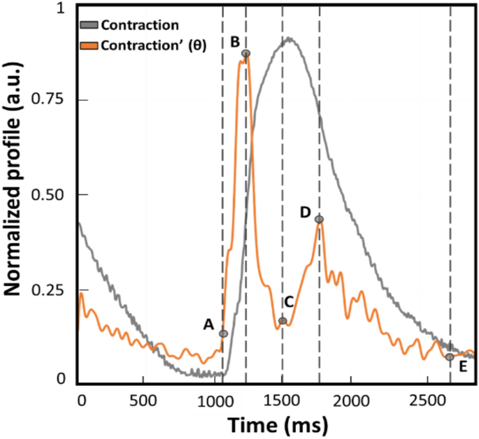
Example of normalized contraction profile (grey trace) and its first derivative named θ (orange trace) obtained with MUSCLEMOTION (benchmark). This represents a qualitative graphical description of the kinematic parameters calculated and compared during the experiments. The time between points A and E is defined as beat duration. The time between points B and D is the distance between the peaks of contraction and relaxation (t[θc−r]). The time between points A and B corresponds to the interval of maximum speed during the contraction phase (t[θc]). Lastly, the time between C and D is defined as the interval of maximum speed during the relaxation phase (t[θr]).
All the videos were recorded with consistent frame rate throughout the experiments and in the same conditions. Moreover, it has to be noted that the profiles reported throughout the work will be indicated as absolute values to avoid misinterpretation and ensure consistency in data representation of the outputs from the three computer vision software. From the absolute of the speed profile, four parameters were calculated to assess any difference in the kinematic evaluation. A representative contraction profile and its first derivate (named as θ) are displayed in Fig. 1 to highlight the parameters calculated on each different software output. The profiles reported were derived from the benchmark MM and normalized. A remark from the authors is the slight temporal anticipation of the speed profile due to the approximation of the ratio of increments from which the first derivate is calculated. As illustrated in Fig. 1, the parameters over the speed profile (orange trace) were selected according to the physiological contraction response (grey profile). The difference between points E and A is defined as beat duration and corresponds to the time elapsing between the 5% of the end of contraction and the onset defined as the first value different from zero. The difference between points B and A is the time required to reach the maximum speed of the contraction phase (t[θc]), as the maximum slope in the ascending phase of the contraction profile. The difference between D and C is the maximum speed reached during the relaxation phase (t[θr]), namely the maximum slope in the descending phase of the contraction. The distance between points D and B is considered the distance between the peaks of contraction and of relaxation (t[θc-r]).
In-silico cardiomyocytes
By kind courtesy of Prof. Sala, a batch of the in-silico cardiomyocyte (CM) videos, used to establish the MM method, was employed to perform the first comparison between the three software. Briefly, the videos were created using Blender software (v2.77, Stichting Blender Foundation) to simulate cardiomyocyte-shaped objects in motion. The in-silico simulations were designed with two different graphical patterns: (i) a grey-based with repetitive black bands present along the structure in both longitudinal and perpendicular directions and (ii) a diffuse phase contrast to simulate highly repetitive pattern of an in-vitro single CM36. The videos were analyzed with two different time-to-peak values (50% and 200% of the baseline value considered 100%) but with constant amplitude of contraction. The software programs were evaluated based on their capability to estimate the correct kinematic stated by MM. Moreover, both qualitative and quantitative comparison of the output parameters was performed over a sample beat, as described above.
Ventricular cardiomyocytes isolation
Single ventricular cells were derived from 6-month-old mice via Langendorff isolation (Louch et al., 2011). All experiments were performed according to the 2010/63/EU Directive and approved by the ethics committee of Humanitas Research Hospital, with code 07/2019. Moreover, the animal experimentation was performed in accordance with the ARRIVE guidelines, and all the authors complied to the above regulations. Briefly, mice were anesthetized with ketamine (100 mg/kg) and xylazine (10 mg/kg) administered via intraperitoneal injection. Mice were placed in dorsal recumbency, and after chest opening, the heart was excised. The aorta was cannulated with a 21-gauge needle and secured to a Langendorff apparatus. Cardiomyocytes were obtained by enzymatic perfusion of the left ventricle with Collagenase Type II (Worthington, LS004177, ≥ 125 units per mg). Hanks Balanced Salt Solution (HBSS 1x, Invitrogen 14,170–088) supplemented with magnesium chloride hexahydrate (1 mmol/L, Merck 442,611), taurine (30 mmol/L, Merck T0625), D-( +)-glucose (15 mmol/L, Merck G5767), magnesium sulfate (1.2 mmol/L, Merck M2643) was made to further process the cells. The digested heart was removed from the apparatus and submerged in stop solution (4% Bovine Serum Albumin, BSA, in supplemented HBSS), and the left ventricle was dissected from the right ventricle and atria. The tissue was gently minced and pipetted to release cells. The cells were filtered through a 100 µm-mesh strainer to avoid contamination with undigested tissue fragments. CMs were sedimented by centrifugation at 120xg for 30 s. The cell pellet was washed 3 times in supplemented HBSS and brought at the correct calcium concentration with gradual additions. Briefly, 10 µL from the stock solution (10 mmol/L of CaCl2 in HBSS) were added in two steps, and a last dilution of 10 µL ultimate the calcium addition, bringing the cells to a final extracellular concentration of 2 µM. The single cell dimensions were measured via Fiji®.
Frequency protocol and single-cell data acquisition
The cell suspension from the tissue isolation was placed on a heated perfusion chamber at 37 °C equipped with silver wires for field stimulation. Cell pacing was generated using the Myopacer Field Stimulator from IonOptix® at 40 V cathodal stimulation. Once settled at the bottom of the chamber, the cells underwent a frequency protocol at the following steps: 0.5 Hz, 1 Hz and 2 Hz; 5 s videos of paced cardiomyocytes were acquired by a high-speed camera (Basler, acA1300-200 um) at 143 fps, using PylonViewer 5 software (Basler, version 5.1.0.12681 64-bit) and an image dimension of 896 pixels × 980 pixels. The hardware used for the acquisition mounted an Intel(R)® CoreTM i7-8750H CPU at 2.20 GHz, RAM 16 GB on Windows 11 Pro, version 22H2. The cells that respected the entire protocol of pacing were analyzed.
Stem cells culture and 3D cardioid formation
Human embryonic stem cells (RUES) were kindly provided by Dr. Elisa Di Pasquale. The stem cells (passage < 30) were seeded on Matrigel®-coated well plates in Essential-8 medium (Gibco™, #A1517001) and, once reached 70–80% of confluency within 3 to 4 days, differentiated into cardiomyocytes. The differentiation was performed via the PSC Cardiomyocyte Differentiation Kit (Gibco™, #A2921201). Briefly, the protocol induced differentiation through sequential refreshment of the three different media in the kit every two days (medium A, B and M). Once in medium M, the cells were refreshed every 2 days. On the 26th day of culture, the cells were purified from all non-cardiomyocytes by MACS PSC-Derived Cardiomyocyte Isolation Kit (Miltenyi Biotec, #130-110-188) as the negative fraction to depletion antibodies. A resuspension of 50.000 cells in DMEM (Gibco™, 11960-044 supplemented with glutamine 1:1000) completed with 10% FBS (Microgem, S1860-500) and 1% P/S (Euroclone, ECB3001D) was seeded into round-bottomed ultra-low attachment 96-well plate. After 4 days, the cells started to form small clusters and within a week began to compact into cardioids (Hofbauer et al., 2021). The medium was partially refreshed every 3 days. The cardioids dimensions were measured via Fiji®.
Frequency protocol and cardioid data acquisition
At day 50 of culture, the cardioids were singularly picked and transferred into a field stimulation chamber (Warner instruments, RC-49MFSH) at 37 °C and 5% CO2, powered by the stimulus generator STG4004-16 mA (Multi Channel Systems MCS GmbH) at 8 V with a step cathodic function, duty cycle 20 ms, and increasing frequencies of 0.5 Hz, 0.75 Hz and 1 Hz. From previous experiments, we observed that the maximum pacing frequency to keep the 1:1 ratio was 1 Hz, leading to an adaptation of the frequency protocol employed in the single cells. Videos of 10 s at 143 fps were recorded using a high-speed camera (Basler, acA1920-155 um), driven by PylonViewer software 6 (Basler, version 6.2.0.8205), running on an Intel® CoreTM i5-9400F, CPU at 2.90 GHz, RAM 16.0 GB, Windows 11 Home, version 21H2, grabbed image dimension of 1000 pixels × 1000 pixels. For each condition, a biological triplicate was assured.
Caffeine and potassium treatments
To assess software sensibility, two substances were added to the sample medium during the frequency protocol described in detail above. Specifically, samples underwent either a controlled increase of extracellular potassium for inducing depolarization (KCl, Sigma-Aldrich P9541) or an addition of caffeine (Sigma-Aldrich W222402) at 10 mmol/L concentration for inducing inotropic response. These concentrations were assessed to be the most effective kinematic-wise based on previous experiments and the literature66,67. Five minutes after the substances administration, videos were recorded and collected for further data analyses, as previously described.
Dataset and supervised machine learning
For each algorithm (MM, CW, and ViKiE), we produced a dataset at each frequency of stimulation in either adult single cells or cardioids for a total of 18 datasets. The treatment factor was considered to be either 10 mmol/L caffeine or 10 mmol/L KCl. The datasets consisted of the 4 kinematic measures (Fig. 1), two time-dependent parameters (the contraction and relaxation peaks magnitude), and the classification label (treated or control). Finally, the rows contained the parameters of each beat. We added the contraction and relaxation peaks magnitude to the set of parameters to have a larger number of features for the classification. The datasets were split into training and testing sets with a ratio of 0.80. In the case of an unbalanced dataset, i.e., composed of an unequal amount of data in one class compared to the other (treated vs control), a re-balancing by sampling a subset of the overrepresented class was made and merged with the underrepresented set.
Machine learning was applied by using random forest (RF) and support vector machine (SVM), the latter with two different kernels (linear and polynomial). RF algorithm was selected because it emerged as the best approach in a study classifying contractile profiles64, whereas the SVM algorithms were selected as commonly used in machine learning. Specifically, SVM with linear and polynomial kernels obtained the highest performance scores. SVM algorithms are classification tools based on four basic concepts: the separating hyperplane, the maximum-margin hyperplane, the soft margin, and the kernel function. The first three elements help to select the optimal hyperplane separating the data points to be classified68, while the kernel function modifies the distribution of the data on the coordinate system to better separate them. RF algorithm is based on an ensemble of decision trees, each working on randomly selected features and a sample of data extracted from the training set69. All the decision trees in the RF perform a classification and, in the end, a majority vote is pooled. The described algorithms were employed to classify the datasets described above. The performance metrics considered in this work were the true positive rate (TPR) (Eq. (1)) and accuracy (Eq. (2)), which are defined according to the values of the confusion matrix, as shown in Table 1.
$${text{TPR}} = {text{TP}}/left( {{text{TP}} + {text{FN}}} right)$$
(1)
$${text{Accuracy}} = left( {{text{TP}} + {text{TN}}} right)/left( {{text{TP}} + {text{TN}} + {text{FP}} + {text{FN}}} right).$$
(2)
Ethics approval
The mice adult ventricular cardiomyocytes were obtained in accordance to the protocol code 07/2019, approved by the ethical committee Directive of Humanitas Research Hospital and according the 2010/63/EU Directive.
- SEO Powered Content & PR Distribution. Get Amplified Today.
- PlatoData.Network Vertical Generative Ai. Empower Yourself. Access Here.
- PlatoAiStream. Web3 Intelligence. Knowledge Amplified. Access Here.
- PlatoESG. Carbon, CleanTech, Energy, Environment, Solar, Waste Management. Access Here.
- PlatoHealth. Biotech and Clinical Trials Intelligence. Access Here.
- Source: https://www.nature.com/articles/s41598-024-52081-9