Human PSC lines
The human PSC lines used in this study are 1) NCRM-1 (RRID:CVCL_1E71) hPSC line from NIH Center for Regenerative Medicine (CRM), Bethesda, USA. 2) ZO1 hPSC line (Mono-allelic mEGFP-Tagged TJP1 WTC, Coriell institute for Medical Research), 3) hPSC F-actin reporter line provided by Catherine Verfaillie, Stem Cell institute Leuven.
Human PSC culture
Matrigel-coated 6 well plates were used to maintain hPSCs cultured to 60–70% confluence. Human PSC colonies were passaged using a treatment of Dispase (Sigma) for 4 m at 37 °C followed by PBS washes. 1 mL of Essential 8 (E8)—Flex Medium Kit (ThermoFisher Scientific) supplemented with 1% Penicillin Streptomycin (GIBCO) and Y-27632 Rock inhibitor (ROCKi) (Hellobio) at 10 μM was used to passage colonies after gentle scraping and agitation with a pipette to break down the colonies. Colonies were passaged 1:6 and incubated in 2 mL of E8-Flex medium supplemented with ROCKi at 10 μM for 24 h. The medium was replaced by 4 mL of fresh E8-Flex and the colonies were incubated for an additional 48 h when they reached 60–70% confluence.
Magnetic nanoparticle (MNP) preparation and magnetic cluster (MagC) labeling with red fluorescent particles
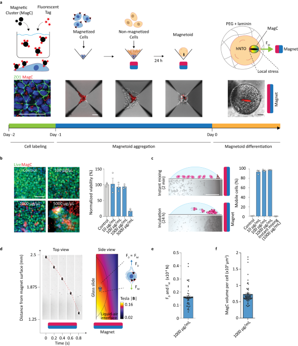
100 mg of Fe3O4 magnetic nanoparticles (MNPs) (Sigma-Aldrich, 20–40 nm) were first weighed under sterile conditions and added to 1 mL of E8-Flex media, in a 1.5 mL Eppendorf tube, resulting in a stock MagC mixture with a concentration of 100 mg/mL. The solution was pipetted thoroughly and subsequently sonicated for 5 m to break apart any aggregation. To label the MagCs, 20 μL (2 mg of MagCs) were taken from the stock mixture, immediately following sonication, and added to 2 mL of E8-Flex medium supplemented with 10 μM of ROCKi. The mixture was then sonicated for 3 m to break up aggregation. Next red fluorescent beads (FluoSpheres Carboxylate-Modified Microspheres, 200 nm, Invitrogen) were diluted 1:10 in E8-Flex supplemented with 10 μM of ROCKi and sonicated for 5 m to break up any aggregation. Subsequently, 5 μL of the diluted fluorescent particles were added to the 2 mL MagC-medium mixture to obtain a final composition of 0.025% v/v (1:4000 dilution of the stock solution). The mixture was immediately sonicated for 3 m to increase MNP-fluorescent particle interaction resulting in efficient labeling of the MagCs. This created a 2× magnetic cluster (MagC) solution.
Magnetization of human induced pluripotent stem cells
Human hPSCs, at a confluence of 60–70%, were washed with PBS three times, followed by the application of 1 mL of TrypLE Express (GIBCO) at 37 °C for 3 m for dissociation. Once dissociated into single cells, 9 mL of DMEM/F12 medium supplemented with 20% FBS (GIBCO) was added for neutralization and TrypLE Express washing. The cells were then centrifuged at 300 RCF for 3 m After discarding the supernatant, a second wash was applied by adding 10 mL of DMEM/F12 medium containing 20% FBS followed by centrifugation at 300 RCF for 3 m. The supernatant was discarded and the cells were resuspended in 1 mL E8-Flex medium supplemented with 10 μM of ROCKi. A cell count was performed and the volume of medium was adjusted to obtain cell density of 500,000 cells/mL. A volume of 1 mL was added to a Matrigel-coated well of a 6-well-plate. Immediately after, 1 mL of the 2× MagC solution was added and gently mixed with the cells using a 1000 μL pipette. The same protocol was followed for the control cells, except the final 1 mL medium addition contained no MagCs. The cells were incubated for 24 h (37 °C, 5% CO2) to obtain mhPSCs and control hPSCs.
Magnetoid protocol
A 24-well AggreWell™400 plate (Stemcell Technologies) was first prepared following the manufacturer’s anti-adherence treatment recommendations. Magnetized and control cells were washed, dissociated, and centrifuged following the above protocol. After a cell count, enough volume of dissociated cells was added to 2.5 mL of E8-Flex medium supplemented with 10 μM of ROCKi to obtain a density of 89,100 cells/mL. A similar procedure was followed for the mhPSCs, however, obtaining 1 mL of E8-Flex medium containing 10 μM of ROCKi and a cell density of 900 cells/mL.
Next, the 24-well AggreWell™400 plate was prepared for cell aggregation. First, 1 mL of mhPSCs was added to a well and aggregated immediately at 300 RCF for 3 m. Subsequently, in the same well, 1 mL hPSCs was added dropwise to the liquid-air interface using a 200 μL pipette. In the control well, 1.01 mL of hPSCs was added directly and topped with 0.99 mL of E8-Flex supplemented with 10 μM of ROCKi. The cells were immediately aggregated at 300 RCF for 3 m.
Once aggregated, another standard 24-well plate was used to house a magnet (Supermagnete, N45, 15 × 15 × 15 mm) with the magnetization axis pointing vertically. The magnet was placed inside one of the wells and covered by the well-plate cover. The well was chosen such that it matched the position the well containing the mhPSCs in the 24-well AggreWell™400 plate. Next, starting from a vertical position of more than 20 cm directly above the 24-well-plate with the magnet, the AggreWell™ was lowered until it was resting securely above the well-plate containing the magnet. The assembly was then moved to the incubator and the cells were incubated (37 °C, 5% CO2) for 24 h.
After the incubation period, the assembly was gently moved out of the incubator and the AggreWell™ was lifted in a vertical manner until it was approximately 20 cm away from the well-plate containing the magnet. This ensured the magnetic aggregates were not magnetically disturbed. 1 mL of media was gently taken out. The magnetic and nonmagnetic aggregates were then separately suspended in the remaining 1 mL of medium using a 1 mL pipette (a wide bore tip should be used to avoid damaging the aggregates). The aggregates were then moved to separate 1.5 mL Eppendorf tubes and centrifuged at 150 RCF for 3 m. The supernatant was removed and 12 μL of differentiation medium was added to each aggregate condition.
A 100 μL 2 kPa Polyethylene glycol (PEG) hydrogel was prepared as previously described16 for each condition. The 10 μL cell suspension16 was replaced by a 10 μL aggregate suspension. 10 μL of aggregate-containing hydrogels were placed in wells of a 96-well plate. For the magnetically actuated magnetoid condition, the border wells were chosen. For the control and magnetoids without magnetic actuation, a different well plate was chosen. The well plates were continuously rotated to prevent organoid aggregation and settling until PEG gelation was visually confirmed16. An additional 20 m was required to ensure complete gelation at room temperature conditions. Subsequently 200 μL of differentiation medium (see below) was added to each well. A rectangular magnet (Supermagnete, N45, 30 × 30 × 15 mm) was placed next to the well plate containing the magnetoid for actuation. The magnet was placed on a 1.5 mm plastic spacer so that it was not directly touching the incubator shelf. The well-plate containing the control and non-actuated magnetoids was placed at least 20 cm away from the magnet to reduce magnetic disturbance.
Human neural tube differentiation magnetization protocol
Organoids were treated immediately after PEG embedding for 3 days with neural differentiation medium comprised of a 1:1 mixture of neurobasal medium (GIBCO) and DMEM/F12 (GIBCO), 1% N2 (GIBCO), 2% B-27 (GIBCO), 1 mM sodium pyruvate MEM (GIBCO), 1 mM glutamax (GIBCO), 1 mM non-essential amino acids (GIBCO) and 2% Penicillin Streptomycin (GIBCO) and supplemented with 10 μM of ROCKi. To induce floor plate identity, organoids were treated from days 3–5 with ROCKi-free neural differentiation medium supplemented with retinoic acid (RA) (Stemcell Technologies) at 0.25 μM and smoothened agonist (SAG) (Stemcell Technologies) at 1 μM. The organoids were subsequently treated with ROCKi-free neural differentiation medium until end point day 11 and the medium was fully refreshed every 2 days. The magnetic field was applied for the entire duration of the 11 day differentiation protocol for all hNTO patterning experiments, except those reported in Supplementary Fig. 9. In Supplementary Fig. 9, to observe the effect of magnetic field removal on pattern stability, we removed the magnet at day 9 and observed FOXA2 expressions at day 11. In a separate experiment, we removed the magnet at day 11 and observed FOXA2 expressions at day 13. In both experiments, the organoids where not subjected to a localized force generated by the MagCs for a duration of 2 days. In these experiments, the differentiation timeline of the unactuated hNTmOs and control organoids was changed accordingly to reflect the same endpoints as the actuated hNTmOs.
Magnetic nanoparticle toxicity study
Fluorescently labeled MagCs were prepared following the MagC labeling protocol to obtain 2× concentration solutions of 20, 200, 2000, and 10,000 µg/mL. The respective fluorescent particle concentration for each condition was adjusted to maintain their ratio to MNPs. Single hPSCs were plated in wells of a 6-well-plate at a density of 100,000 cells/mL in a volume of 1 mL of E8-Flex supplemented with 10 μM ROCKi. Next 1 mL of the 2× MagC solutions was added to the respective wells and mixed gently with a 1000 μL pipette. The cells were incubated for 24 h, at which point the medium was replaced with ROCKi-free E8-Flex medium and incubated for an additional 48 h. Media change was done carefully to not disturb the MagCs in the wells. Cells were then washed, dissociated, centrifuged and resuspended in 1 mL of E8-Flex medium supplement with 10 μM of ROCKi. A cell count was performed and the total amount of cells per condition was evaluated and normalized to that of the control condition. These values were reported to compare the toxicity of MagCs on hPCS. In separate wells with intact colonies, Calcien AM (Thermofisher) was used to visualize live cells in control and magnetized conditions. The cells were then fixed in paraformaldehyde (PFA 4%, Sigma-Aldrich) for 2 h and gently washed with PBS. The cells were then treated with a permeabilization and blocking solution comprised of 0.3% Triton X (PanREAC AppliChem) and 0.5% BSA (Sigma–Aldrich) in PBS for 30 m. Hoechst was then used to visualize DNA and applied at a concentration of 1:2000 in permeabilization and blocking solution for 2 h at 4 °C followed by 3 PBS washes. Representative images were then obtained using an inverted microscope (Zeiss Axio Observer Z1; Carl Zeiss MicroImaging) equipped with a Colibri LED light source and a 10× air objective.
Magnetic cluster localization
ZO1 hPSCs were magnetized using a 1 mg/mL MagC solution following the magnetization protocol. The cells were then imaged using confocal microscopy (Leica SP8 DIVE, Leica Microsystems). 3-D reconstructed images were generated from image stacks to demonstrate the localization of MagCs and ZO1 (apical).
Magnetic cluster size analysis
MagCs were prepared and labeled as described in the above protocol to yield a 2 mg/mL 2×-2 mL solution. A volume of 5 μL was taken and added to 1 mL of DMEM medium and sonicated for 3 m. A 100 μL droplet of the mixture was taken and added to a glass slide. The droplet was imaged using an inverted microscope (Zeiss Axio Observer Z1; Carl Zeiss MicroImaging) equipped with a Colibri LED light source and a 40× air objective. MagCs sizes were assessed using the particle analysis function in ImageJ.
Magnetic cluster position analysis
1% mhPSC-hNTmO at day 11 were analyzed for the position of their respective MagCs. To obtain a dimensionless analysis for the position of the MagC, for every magnetoids the brightfield image was scaled and projected onto a circular hypothetical organoid while retaining the magnet direction. The MagC shape was then segmented, its position retained and transformed into a binary grayscale image where the MagC shape was attributed a gray scale value of 10 (ImageJ). All MagC images were then projected onto the same space and the intensities were summed. Intensity variation was then color-coded for position density were higher intensities reveal regions most likely to be occupied by MagCs.
Magnetization efficiency
Magnetized hPSCs were prepared with final MagC concentrations of 10, 100, and 1000 μm/mL following the magnetization protocol. After 24 h incubation, the cells were washed, dissociated, centrifuged and resuspended in 1 mL of E8-Flex medium supplement with 10 μM ROCKi. A 100 μL droplet of the mixture was taken and added to a glass slide. The glass slide was placed under an inverted microscope (EVOS, Invitrogen) and visualized using a ×4 objective. An image was acquired showing the cell positions as they settled towards the glass slide. A magnet (Supermagnete, N45, 15 × 15 × 15 mm) was placed at a distance not greater than 1 mm from the droplet edge. After 2 m, a second image was taken of the same droplet and position. Using ImageJ, a visual comparison determined the percentage of cells that underwent magnetophoresis. Two other conditions were also assessed, 1) control unmagnetized hPSCs, and 2) hPSCs that had been instantly mixed with a final MagC concentration of 1000 μg/mL, following magnetization protocol.
Magnetic simulations (FEMM) and force estimation
The program Finite Element Method Magnetics (FEMM, version 4.2) was used to conduct two-dimensional axisymmetric magnetics simulations to compute the magnetic field produced by the various magnets used in the study. First, the profile area of the used magnet was constructed and assigned a NdFeB N45 material property from the built-in FEMM material library. The well plate, the PEG hydrogel and the organoid tissue were all considered permeable to the magnetic field and thus ignored in the simulation. All unfilled spaces around the magnet was assigned the material properties of air from the built-in FEMM material library. Standard meshing was chosen prior to running the simulation.
To evaluate the magnetic force produced by MagCs in magnetoids, we first evaluated the field strength within the first well of a 96 well plate and where magnetoids are to be expected. We found the magnetic field produced by the magnet to vary between 0.2 and 0.1 T within the well, which is a range below the magnetic field strength required for Fe3O4 nanoparticle saturation magnetization. The magnetic field strength is therefore considered weak and the magnetic moment linearly varies with the applied magnetic field37. To calculate the force, a straight line was trace from the corner of the magnet and extended outwards into the air environment. The line length spanned the entire length of a well-plate and the magnetic field values, ({{{{{bf{B}}}}}}), were extracted in Tesla. To estimate the magnetic force, we first evaluated the gradient of the squared field, (partial {{{{{{boldsymbol{|}}}}}}{{{{{bf{B}}}}}}{{{{{boldsymbol{|}}}}}}}^{2}/partial {{mbox{y}}}), along the length of the line section. The magnetic force density, ({{{{{{bf{f}}}}}}}_{{{mbox{m}}}}{{{{{boldsymbol{=}}}}}}({upchi}_{{{{mbox{Fe}}}}_{3}{{{mbox{O}}}}_{4}}/2{upmu}_{{{mbox{o}}}})partial {{{{{{boldsymbol{|}}}}}}{{{{{bf{B}}}}}}{{{{{boldsymbol{|}}}}}}}^{2}/partial {{mbox{y}}}), was then calculated where the magnetic volume susceptibility of Fe3O4 was assumed for MNPs as ({upchi}_{{{{mbox{Fe}}}}_{3}{{{mbox{O}}}}_{4}}{{mbox{=}}}9448{{mbox{.}}}8) and the permeability of free space ({upmu}_{{{mbox{o}}}}=4{uppi}times {10}^{-7}). Each well directly facing the magnet (e.g. six adjacent wells that form a column on a 96-well-plate) was divided into six horizontal tranches with equal thickness. Each tranche was assigned one ({{{{{{bf{f}}}}}}}_{{{mbox{m}}}}) value using the simulation data and based on the distance separating the centroid of the tranche to the magnet surface. For any magnetoid in a tranche, the magnetic force ({{{{{{bf{F}}}}}}}_{{{mbox{m}}}}=,{{{{{{bf{f}}}}}}}_{{{mbox{m}}}}{{{mbox{V}}}}_{{{{mbox{Fe}}}}_{3}{{{mbox{O}}}}_{4}}), where ({{{mbox{V}}}}_{{{{mbox{Fe}}}}_{3}{{{mbox{O}}}}_{4}}) was the volume of the MagC. In this way, the force generated by any MagC in any magnetoid located at any distance away from the magnet surface could be estimated. To estimate the MagC volume, we tested three volume estimation methods 1) cylindrical, 2) elliptical and 3) pixel-depth. In the cylindrical method, the MagC outline is firs traced and the long, a, and short, b, axis of the best fitting ellipse are evaluated. The volume was then evaluated a Vcylindrical = V = πa(b/2)2. The elliptical volume followed the same procedure as the cylindrical method but where Velliptical = V = (4/3)πab2. In the pixel-depth method, the MagC outline was traced, and the corresponding area, A, was evaluated. Next, the widths at the beginning (evaluated at one quarter the length of the long-axis away from the MagC end), middle and end (evaluated at one quarter the length of the long-axis away from the other MagC end) of the MagC were evaluated and averaged, wavg. The MagC volume was then evaluated as Vpixel-depth= Awavg. Although elliptical geometries are supported by theory, we observed that the MagCs do not strictly adhere this shape as they appear more cylindrical with tapered ends. This may be attributed to the assembly of smaller MagC ellipses to form larger structures. We therefore consider this elliptical method to be an underestimation. Indeed, when comparing the different volume estimation methods we found that the cylindrical and pixel-depth methods resulted in similar volume values with a pixel-depth to cylindrical volume ratio on average ~0.93. By contrast, the elliptical to cylindrical volume ratio on average ~0.67. From visual assessment of MagC shapes, and knowing that two independent methods results in similar volume estimation values, in this study we considered the cylindrical volume estimation method as it required less input parameters that the pixel-depth method. For magnetoids where multiple MagCs appear, such as in the case of 5% and 25% mhPSC-magnetoids, the volume for each MagC is estimated then summed to obtain a total MagC volume per magnetoid. The force is then estimated based on this summed volume, i.e. the obtained force values are that of the cumulative forces from each of the MagCs in the magnetoid. In the 1% and 0.5% mhPSC-magnetoid cases, the majority of magnetoids had one MagC.
Magnetic force and single-cell fate correlation
The magnetic force was measured as detailed above. Next the distance that separates the centroid of FOXA2+ or PAX6+ nuclei and that of the MagC in the was measured. Both the distance and force were then reported in a correlation plot (Supplementary Fig. 4). Only distances toward the biased zones for each fate (FOXA2—towards the magnet, PAX6—away from the magnet) were reported.
Magnetic force analysis on single cells
Magnetized hPSCs were prepared with a final MagC concentration of 1,000 μm/mL following the magnetization protocol. After 24 h incubation, the cells were washed, dissociated, counted, centrifuged, and resuspended in E8-Flex medium supplement with 10 μM ROCKi with a volume to obtain (sim 10-100{{mbox{cell}}}/upmu{{mbox{L}}}). This low concentration reduced cell-cell flow perturbation. A glass slide was prepared where a magnet (Supermagnete, N45, 3 × 3 × 3 mm) was glued in place with the magnetization axis aligned with the slide’s long axis. The glass slide was then mounted onto the stage of an inverted microscope (Zeiss Axio Observer Z1; Carl Zeiss MicroImaging, 5× objective). Next, 100 µL of the cell suspension was placed onto a glass slide. As the cells underwent magnetophoresis, they began to move through the medium toward the magnet surface and a video (5 frames per second) using the brightfield channel was taken. Using ImageJ, the distance (measured between forward cell edges in consecutive frames) traveled for each cell between frames was measured and divided by 0.2 s to obtain a velocity u (~100 µm/s). For a cell radius R of ~10 µm, this velocity resulted in a Reynold’s number (ll)1, suggesting Stoke’s flow conditions where FD = FM where FD is the drag force and FM is the magnetic force acting on the MagCs. For each cell, ({{{{{{bf{F}}}}}}}_{{{mbox{D}}}}=6{uppi}upmu{{mbox{R}}}{{{{{bf{u}}}}}}), where µ = 8.9 · 10–4 Pa s is the dynamic viscosity of water, R is the cell radius assuming a spherical geometry, u is the calculated cell velocity between frames. The magnetic field produced by the 3 × 3 × 3 mm magnet was then simulated and a force density plot was generated. Knowing FM and using the force density plot we could estimate the volume of MagCs attached the cells ~7.3 × 103 µm3. When comparing this value to those measured for MagCs in magnetpoid, we saw a difference, suggesting that in addition to the assumed ~1 mhPSCs that is integrated per magnetoid for the 1% mhPSC condition, other unbound MagCs can also find their way into the cellular construct during the aggregation step. It is therefore more accurate, for the purpose of evaluating forces in magnetoids, to estimate the MagC volume in magnetoids directly from images and not simply assume a volume based on the single cell FM measurements. These single-cell magnetophresis experiments inferred proper attachment of the MagCs to the cells.
Short-term magnetoid actuation
A short-term magnetic actuation was conducted on magnetoids embedded in 2 kPa PEG hydrogels, prepared as discussed above and plated in a 96 well plate. Day 11 hNTmOs were observed using an inverted microscope (EVOS, Invitrogen). A magnet (Supermagnete, N45, 15 × 15 × 15 mm) was placed at a ~ 45° angle (directly next to the adjacent well) with the magnetization axis perpendicular to the plate edge. This setup still allowed MagCs to reorient toward the magnet. An image was then taken of the magnetoid every 5 s for 30 s. Using ImageJ, the displacement of the tissue around the MagC as it reorients towards the magnet was traced and measured by choosing a visible and trackable tissue feature on the brightfield channel. We measured the displacements caused by whole magnetoid rotation and subtracted these from the tissue displacements. The field of view was divided into an array of tissue sections and the displacements, dtissue, in each tissue section were normalized to the displacement of the part of the MagC, dM, in that row to provide a dimensionless displacement value d*. The distance, x, from the centroid of each tissue section to the edge of the MagC in the same row was normalized to the displacement of the part of the MagC in that row to provide a dimensionless coordinate value c*. A d*-c* correlation and heatmap was then reported.
Long-term magnetoid actuation
A similar setup as the one discussed above was used. However, here the magnet was placed for longer durations of 5, 30, 60, and 120 m under incubation conditions of previously magnetically actuated day 11 hNTmOs. At time t0 without the magnet placement, the reference angle of the MagC was imaged. At every subsequent time point, the magnet was taken away and the new MagC angle was imaged. The recoil angle difference, α, was calculated by subtracting the reference angle (original position) from the new angle (final position) and was then reported.
Growth and proliferation studies
To determine the size of hNTmOs, day 11 magnetoids were imaged using an inverted microscope (EVOS, Invitrogen). Using ImageJ, the projected area of organoids was traced and converted to an equivalent diameter assuming a circular area.
To determine the biased growth of magnetoids when compared to control or unactuated magnetoids, all organoids brightfield images were taken at days 1 and 11. A contour line was traced to mark the organoid boundary at days 1 and 11 and the images were superimposed using non-mobile reference points in the surrounding matrix as anchor points. Next, a line section, Pm, was traced connecting the closest point to the magnet surface of the contours at days 1 and 11. A similar line section, Pa, was traced to connect the furthest point to the magnet at both days. The ratio of the growth towards the magnet, Pm, and growth away from the magnet, Pa, was calculated where a value <1 and >1 indicated biased growth away and toward the magnet respectively while a value ~1 represented an unbiased growth direction.
To determine the proliferation bias, day 11 hNTOs and hNTmOs were fixed and stained with EdU and images were taken using an inverted microscope (Zeiss Axio Observer Z1; Carl Zeiss MicroImaging, 10× objective). For all cases, a line segment dividing the organoid into two halves and passing through the organoid centroid was traced. The average EdU intensity in the halves facing the magnet, EdUm, were normalized to that of the respective halves facing away from the magnet, EdUa, where a value <1 and >1 indicated biased proliferation away and toward the magnet respectively while a value ~1 represented an unbiased proliferation direction.
To investigate the cell density bias, the averaged Hoechst signal from organoid halves from day 11 hNTOs and hNTmOs was analyzed in the same way as the EdU analysis. A Hoechst intensity ratio <1 indicated less cells in the organoid half facing the magnetic and a value >1 indicated less cell density in the organoid half facing away from the magnet, while a value of ~1 represented a balanced cell density between the halves of the organoid.
Fate specification and patterning studies
The induction and patterning efficiencies of FOXA2, NKX2.2, OLIG2, NKX6.1, ISL1/2, and PAX6 were visually inspected across the various conditions using an inverted microscope (Zeiss Axio Observer Z1; Carl Zeiss MicroImaging, 10× objective). First organoids were fixed with 4% PFA for 2 h followed by PBS washing and then permeabilization and blocking using a solution of 0.3% Triton X (PanREAC AppliChem) and 0.5% BSA (Sigma-Aldrich) for 30 min. Next, primary antibodies suspended in blocking and permeabilization solution were applied to the samples for 24 h. The following primary antibodies were used in this study, FOXA2 (Santacruz (sc-374376), mouse monoclonal, dilution 1:200), NKX2.2 (DSHB (DSHB − 74.5A5), mouse monoclonal, dilution 1:200), OLIG2 (R&D systems (AF 2418), goat polyclonal, dilution 1:200), NKX6.1 (DSHB (DSHB – F55A10), mouse monoclonal, dilution 1:200), ISL1/2 (DSHB (DSHB − 39.4D5), mouse monoclonal, dilution 1:200), TUBB3 (Biolegend (802001), rabbit polyclonal, dilution 1:200), PAX6 (Biolegend (901301), rabbit polyclonal, dilution, 1:200). The samples were subsequently washed three times using PBS over a period of 24 h. Immunolabeling was then performed using secondary antibodies suspended in blocking and permeabilization solution for an additional 24 h. The following secondary antibodies were used in this study, Alexa Fluor 555 (Invitrogen (A-31570), donkey polyclonal, donkey anti mouse, dilution 1:500), Alexa Fluor 647 (Invitrogen (A-31573), donkey polyclonal, donkey anti rabbit, dilution 1:500), Alexa Fluor 647 (Invitrogen (A-21447), donkey polyclonal, donkey anti goat, dilution 1:500). The samples were subsequently washed three times using PBS over a period of 24 h before imaging.
Pattering efficiencies of FOXA2, NKX2.2, OLIG2, NKX6.1, ISL1/2, and PAX6 in organoids were assessed as previously reported16. Briefly, fluorescent images were assessed using ImageJ to obtain the area of the expression region of the fate as well as the average intensity of the expression in that area. Next, the projected area of the entire organoid or magnetoid was evaluated and an average intensity of the fate expression was obtained. We next evaluated the area ratio (AR) where the fate expression area was divided by the organoid area. We also evaluated the intensity ratio (IR) where the average fate intensity of the expression region was divided by that of the organoid or magnetoid area. The fate was considered as scattered for (1) AR > 0.5, and (2) AR < 0.5 but IR < 20%. By contrast, the fate expression was found to be pattered for AR < 0.5 and IR > 20%. We note that one of the biological replicates in the unactuated hNTmO cases (Fig. 5a) yielded no patterning of PAX6 expressions. We believe this to be an outlier as all other 3 biological replicates cluster together.
To evaluate the percentage of dorsoventral patterning we assessed the expression of NKX6.1 (ventral fates) and PAX6 (intermediate fates) in the same organoid and reported the overall fraction of double positive organoids.
To interrogate expression phenotypes for each of the markers, the marker expression image was scaled and projected onto a circular hypothetical organoid while retaining the original orientation. For each marker, the hypothetical organoid images were projected onto the same space and the intensities were integrated. Intensity variation was then color-coded. Higher intensities revealed regions with highest marker positional bias in the organoid space across 50 to 100 organoids from 3 to 5 biological replicates. To quantify the marker directional bias upon internal force generation, inverted microscopy images were assessed, in a similar manner as for EdU stains, for each of the markers separately.
To investigate pattern organization with reference to the magnetic field direction, we evaluate the projected intensity profiles of FOXA2, NKX6.1, NKX2.2, OLIG2 and PAX6 of the integrated marker expression every 30° from −90° to 90° from the original organoid orientation. The profiles were first normalized then compared to an ideal square intensity pattern and a correlation was established using the corrcoef function MATLAB (R2018a, The MathWorks Ink.). A correlation heatmap was generated using the R (version 4.1.0) package heatmap.2 using RStudio (RStudio Team (2020). RStudio: Integrated Development for R. RStudio, Inc., Boston, MA URL http://www.rstudio.com/). To visualize the enhanced pattern organization in magnetoids we merged the top 20% of the integrated expressions of FOXA2, NKX6.1, OLIG2, and PAX6 fates and reported their profiles at the original organoid orientation.
To evaluate the magnetic field effect, MagC-free hNTOs were subjected to a magnetic field similar to the hNTmO case. The cytoarchitecture and FOXA2 and PAX6 induction rates were then evaluated.
Quantification and statistical analysis
Two-way ANOVA statistical tests and unpaired two-tailed t test with corrections were used where appropriate with a 95% confidence interval (GraphPad Prism 6, Version 6.01, GraphPad Software, Inc.). Statistical significance was considered for all comparisons with p < 0.05. Microsoft® Excel® for Microsoft 365 MSO (Version 2212) was used for fate induction and patterning quantifications.
Reporting summary
Further information on research design is available in the Nature Portfolio Reporting Summary linked to this article.
- SEO Powered Content & PR Distribution. Get Amplified Today.
- PlatoData.Network Vertical Generative Ai. Empower Yourself. Access Here.
- PlatoAiStream. Web3 Intelligence. Knowledge Amplified. Access Here.
- PlatoESG. Automotive / EVs, Carbon, CleanTech, Energy, Environment, Solar, Waste Management. Access Here.
- PlatoHealth. Biotech and Clinical Trials Intelligence. Access Here.
- ChartPrime. Elevate your Trading Game with ChartPrime. Access Here.
- BlockOffsets. Modernizing Environmental Offset Ownership. Access Here.
- Source: https://www.nature.com/articles/s41467-023-41037-8