Stem Cell

Common and divergent gene regulatory networks control injury-induced and developmental neurogenesis in zebrafish retina – Nature Communications

Time Stamp: December 19, 2023 7:00 PM
Source Node: 395481

Ethics statement

All zebrafish experiments were performed in accordance with the regulations of University of Notre Dame (A3093-01). All the experiment protocols were approved by the University of Notre Dame (21-02-6420 and 21-02-6437) and Johns Hopkins University School of Medicine.

Zebrafish husbandry

Adult albino^b4/b4 ^65,66, mmp9^mi5003 mutant fish³⁶, and transgenic albino Tg(gfap:EGFP)^nt11¹⁹ zebrafish (Danio rerio, AB strain) used in this study were bred and maintained in the Freimann Life Science Center Zebrafish Facility at the University of Notre Dame in accordance with standard operating policies and procedures^2,36. The fish were kept at a temperature of ~26.5 °C and 30% humidity, with a 14-h light, 10-h dark cycle⁶⁷. Tg(gfap:EGFP)^nt11 was used to label the MG by expressing GFP¹⁹. All the zebrafish used in this study were adults between 6 and 12 months old or embryos. Prior to any experiments, the fish were anesthetized or euthanized using 1:1000 or 1:500 2-phenoxyethanol (Sigma), respectively. Animals of both sexes were used in approximately equal numbers for these studies.

Retinal damage and EdU labeling

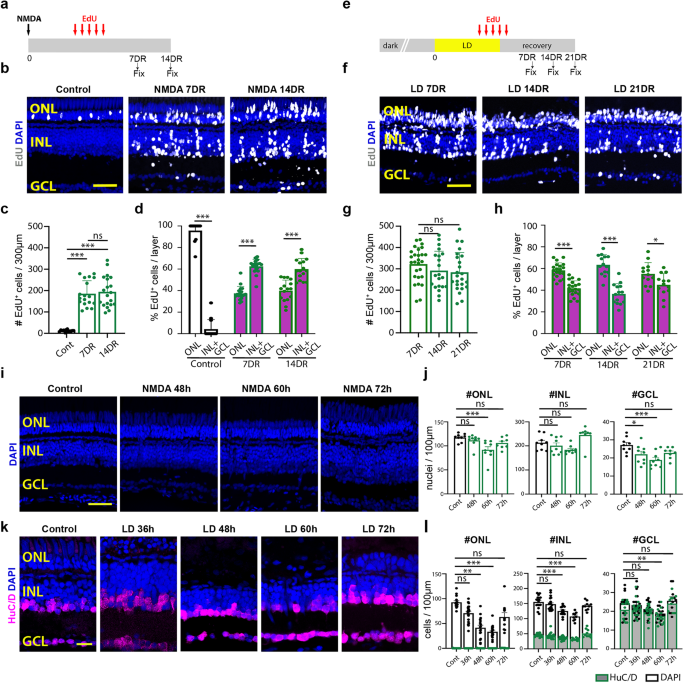
Phototoxic treatment that causes photoreceptor ablation was used to initiate a regenerative response in the zebrafish retina^2,68. All fish subjected to light damage were dark-adapted for 2 weeks and then placed adjacent to intense fluorescent lights for 96 h. The temperature of the fish tanks was regularly monitored and maintained at 34 °C. After 96 h, the fish were returned to the animal facility with a normal light/dark cycle and maintained for 7, 14, or 21 days recovery (DR).

N-methyl-D-aspartate (NMDA, Sigma M3262) was administered to normal light/dark cycled fish via an intravitreal injection of 0.3 µl 100 mM NMDA solution in sterile PBS with a Hamilton syringe (Hamilton, 2.5 µl Model 62 RN SYR, 87942), followed by placing the tanks in a dark incubator at 33 °C for 96 h, after which the tanks were moved back into a normal light/dark cycle for 7 or 14 days recovery.

EdU (5-Ethynyl-2′-deoxyuridine, Life technologies A10044) was administered intraperitoneal via⁶⁸. Fish were anesthetized using 1:1000 2-phenoxyethanol and immobilized under a paper towel in a petri dish. Then, using an insulin syringe equipped with a 30-gauge needle, ~20 µl 1 mg/ml EdU in water was injected intraperitoneally into each zebrafish at 60, 72, 84, 96 and 108 h after damage. The retinal tissues were harvested at either 3, 7, 14, or 21 days recovery.

In vivo morpholino-mediated gene knockdown

Conditional adult retinal morphants were generated essentially as described previously^44,45. Prior to light treatment, fish were anesthetized in 1:1000 2-phenoxyethanol, the outer cornea membrane of the left-eye was removed with Dumont #5 forceps, an incision was then made though the inner cornea in the ventral-caudal aspect of the pupillary margin using a #11 scalpel, and 0.2–0.3 µl of morpholinos (Gene Tools, LLC) at a concentration of 1 mM were injected into the posterior segment using a 2.5 µl Hamilton syringe. Morpholinos that do not target any known zebrafish genes (Standard Control), as well as one targeting pcna, which blocks MG proliferation, were used as negative and positive controls, respectively. Morpholinos were electroporated into the retina using platinum electrode tweezers with a CUY21EDIT Square Wave Electroporator (Nepa Gene Company Ltd.), delivering two 50 msec pulses, separated by a 1 s pause, at 0.75 Volts, resulting in the current of 0.05 Amperes. The electrodes were used to prolapse the eye out of the socket, with the anode in contact with the cornea, and the cathode positioned 2 mm behind the dorsal part of the eye. Successful electroporation was confirmed by the presence of lissamine fluorescence within the retinal cells using microscopy. For the embryos conditional morpholinos mediated knock-down experiments, the morpholinos were diluted to 1 mg/ml in 1x Danieau buffer. Wild-type or Tg(gfap:EGFP)^nt11 embryos were injected with 5 ng of morpholinos at the one-cell stage⁶⁹.

Morpholino sequences used were:

Standard Control: 5’ CCTCTTACCTCAGTTACAATTTATA 3’ (Gene Tools, LLC), anti-pcna: 5’ TGAACCAGACGTGCCTCAAACATTG 3’ ⁴⁵, anti-foxj1a: 5’ CATGGAACTCATGGAGAGCATGGTC 3’⁷⁰, and anti-mmp9: 5’ ACTCCAAGTCTCATTTTGAGTCGCA 3’ (Gene Tools, LLC).

Tissue fixation and cryosectioning

Tissues for immunocytochemical analyses were collected at specified time points by euthanizing zebrafish in 1:500 solution of 2-phenoxyethanol, followed by ocular enucleation using #5/45 Dumont forceps (Supplier). The eyes were floated in 1x Phosphate-Buffered Saline (PBS) solution, and a circular opening, approximately the size of the pupil, was made in the cornea using micro-scissors, creating an eye cup. The eye cups were fixed at room temperature (RT) in 4% paraformaldehyde, using a pH shift technique to preserve the cytoskeletal structure and avoid the cellular swelling that is typically associated with standard paraformaldehyde fixation at 4 °C⁷¹. Briefly, the tissues were fixed at RT for 5 min in 80 mM HEPES, 2 mM EGTA, 2 mM MgCl₂· 6H₂O, 4% PFA, pH 6.8–7.2, followed by 30 min in 100 mM Na₂B₄O₇· 10H₂O, 1 mM MgCl₂· 6H₂O, 4% PFA, pH 11. The eyes were washed in 1x PBS at RT and dehydrated in a 15% sucrose solution at 4 °C overnight. The eyes were then placed in a 2:1 solution of PolyFreeze Tissue Freezing Medium (TFM) (Sigma-Aldrich) and 30% sucrose for 24 h at 4 °C. Finally, the eyes were arranged in the dorsal-ventral plane in 100% TFM, frozen, and stored at −80 °C. Frozen tissue blocks were sectioned using a Thermo Scientific Microm HM550 Cryostat at −23 °C, producing 14 µM serial sections that included the optic nerve and both the dorsal and ventral crescent. Retinal sections were collected on SuperFrost glass slides (VWR 48311-703), dried for 30 min on a slide warmer at 50 °C, and stored at −80 °C for future immunohistochemical staining.

Immunohistochemistry

Retinal sections were processed for immunohistochemistry by drying the slides at 50 °C for 20 min and followed for 3 washes in 1x PBS^2,68. Sections were blocked for 1 h in blocking buffer (1x PBS, 4% normal goat serum, 0.4%Triton X-100, 2% DMSO). When anti-PCNA primary antibodies were used, an extra heat-induced antigen retrieval step was performed. Prior to blocking, slides were immersed in a 10 mM sodium citrate, 0.05% Tween 20, pH 6 solution, and heated for 25 s in a microwave at maximum power to nearly reach the boiling point. The slides were heated for another 7 min using the microwave at 10% power in periodic 20–25 s bursts to maintain near-boiling temperature. The slides were cooled for 30 min at RT and washed 2 × 5 min in 1x PBS before proceeding to the blocking step.

The following primary antibodies were used: mouse anti-PCNA monoclonal antibody (Sigma P8825, 1:500 dilution), rabbit anti-GFAP (Dako Z0334, 1:300 dilution), mouse anti-HuC/D monoclonal antibody (Invitrogen A21271, 1:300 dilution), mouse anti-4c12 monoclonal antibody (gift from Dr. Fadool, Florida State University, 1:200 dilution), rabbit anti-PKCa (Sigma Life Science P4334, 1:300 dilution), rabbit anti-UV cone opsin⁷², 1:1000 dilution), rabbit anti-green cone opsin⁷², 1:500 dilution), mouse anti-Zpr1 monoclonal antibody (ZIRC, 1:200) rabbit anti-Lcp1 (GeneTex GTX134697, 1:500). Secondary antibodies (diluted 1:500) included: goat anti-mouse 488 (Life Technologies A11029), goat anti-mouse 594 (Life Technologies A11032), goat anti-mouse 647 (Life Technologies A21236), goat anti-rabbit 488 (Life Technologies A11034), goat anti-rabbit 594 (Life Technologies A11037), goat anti-chicken 488 (Life Technologies A11039).

Confocal microscopy and quantification

A Nikon A1R HD inverted confocal microscope at the University of Notre Dame Integrated Imaging Facility was used to capture serial optical sections of retinal slices using 40x and 60x oil-immersion objectives. Z-stacks of ~10 µm from the central dorsal retinal tissue were captured using NIS-Elements (RRID:SCR_014329). The resulting images were analyzed as either single optical sections or maximum z-stack projections (where appropriate) using ImageJ/FIJI⁷³. For the colocalization experiments, single optical sections were used. We increased the saturation of the Gfap and 4c12 channels to increase the cell body staining to determine colocalization with EdU.

Statistical analysis

The resulting data were analyzed using GraphPad Prism version 9. Student’s t test for single pairwise comparisons with control or one-way or two-way analysis of variance followed by Dunnett’s or Bonferroni’s post hoc test for multiple comparisons. The statistical significance is indicated in each graph as follows: * for p ≤ 0.05, ** for p ≤ 0.01, *** for p ≤ 0.001, or ns for not significant difference.

ScRNA-Seq of methanol-fixed retinal cells

Zebrafish retinas (4–6 retinas from 4–6 fish) were collected at different time points after NMDA and LD treatments. Retinal cells were dissociated and fixed in −20 °C methanol and stored in −80 °C freezer until used. Fixed cells were recovered and subjected to 10x Genomics Single-Cell system as described previously⁴¹. Libraries were prepared and sequenced on Illumina NovaSeq at ~500 million reads per library.

Multiome analysis of frozen retinal tissues

Zebrafish retinas (4–6 retinas from 4–6 fish) were collected at different time points after NMDA and LD treatments, and flash-frozen in dry ice for ~15 min before being transferred to a −80 °C freezer for storage. Nuclei were extracted from frozen retinal tissues according to 10xMultiome ATAC + Gene Expression (GEX) protocol (CGOOO338). Briefly, frozen retinal tissues were lysed in ice-cold 500 ml of 0.1X Lysis buffer using a pestle and incubated on ice for 6 min totally. Nuclei were centrifuged, washed 3 times and resuspended in 10xMultiome nuclei buffer at a concentration of ~3000–5000 nuclei/ml. Nuclei (~15k) then were loaded onto 10x Genomic Chromium Controller, with a target number of ~10 K nuclei per sample. RNA and ATAC libraries were prepared according to the 10xMultiome ATAC + Gene Expression protocol and subjected for Illumina NovaSeq sequencing at ~500 million reads per library.

Single-cell muti-omics analysis

Preprocessing

The multi-omic sequencing files were processed for demultiplexing and analyzed using Cell Ranger ARC v2.0. The genes were mapped and referenced using the zebrafish reference genome DanRer11. To address potential ambient RNA contamination in the cell-by-gene expression matrix, we employed scAR⁷⁴ module from scvi-tools⁷⁵ with default parameters for ambient RNA cleaning for each sample.

Filtering barcode doublets and low-quality cells for each sample

For snRNA-seq injury analysis, the cell-by-genes matrices were converted to Seurat v3 objects⁷⁶. Doublet cells were identified using the solo module⁷⁷ of scvi-tools. Cells were filtered out if their Solo doublet score were greater than zero. Furthermore, cells with low RNA counts (nCount_RNA < 500) as well as cells with high RNA counts (nCount_RNA > 50,000) were also filtered out as low-quality cells. For snATAC-seq analysis, the fragment files were initially converted to ArchR⁷⁸ objects with default parameters. We only kept the cells which passed quality control in the scRNAseq datasets. Additionally, the cells were further filtered out if their doublet enrichment score were greater than 2. For the development multi-omics datasets, we used the same methods to filter out low-quality cells. However, we only kept cells that passed quality control in both the snATAC-seq and scRNA-seq.

Clustering, visualization, and identification of cell types

The clustering analysis was conducted on the combined dimensional space obtained from both the RNA and ATAC single-cell matrices. Initially, the RNA expression matrix was incorporated into the ArchR project using the “addGeneExpressionMatrix” function. Subsequently, dimension reduction was separately applied to the cell-by-bin matrix and the cell-by-gene matrix within the ArchR project using the “addIterativeLSI” function. The resulting reduced dimensions were then merged into a new dimension called “LSI_Combined” using the “addCombinedDims” function. Finally, clustering was performed using the “addClusters” function with a resolution of 1.5, taking into account the “LSI_Combined” dimensions. To visualize single cells, the UMAP embeddings were calculated using the “addUMAP” function in ArchR with the first 10 “LSI_Combined” dimensions.

To infer cell types, the existing zebrafish scRNA-seq data⁴¹ were utilized for interpreting our snRNA-seq cell types using the CCA (canonical correlation analysis) integration method in the Seurat package⁷⁹. Firstly, the zebrafish scRNA-seq data were downloaded and converted into Seurat objects. Secondly, for each snRNA-seq sample, the anchors between them were identified using the “transfer.anchors” function, and the “TransferData” function was used to obtain the cell type prediction results for each cell. Cells with a prediction score <0.5 were further filtered out, and each cluster was annotated based on their predicted cell types. To further identify precursor cell clusters, the clusters in each major cell type between the control and injury datasets were compared. Clusters that existed in the injury dataset but not in the control dataset were selected as precursor cell clusters and were further confirmed using specific precursor cell markers.

Generating fixed-width and non-overlapping peaks

Fixed-width 501 bp peaks were called for each cell type in both the injury and development datasets by MACS2⁸⁰ in ArchR package. Subsequently, these peaks were merged using an iterative method to retain the most significant peak among overlapping peak sets. The function “addReproduciblePeakSet” was utilized for this calling and merging process. Following that, the peak matrix was generated for each dataset using the function “addPeakMatrix” with the following parameters: ceiling = 4 and binarize = FALSE.

Single-cell RNA-seq data analysis

Preprocessing

The scRNA sequencing files were processed for demultiplexing and analyzed using Cell Ranger. The genes were mapped and referenced using the zebrafish reference genome DanRer11. To address potential ambient RNA contamination in the scRNA-seq expression matrix, we employed SoupX⁸¹ with default parameters for further ambient RNA cleaning for each sample.

Quality control of scRNA-Seq data for each sample

The cell-by-genes count matrices were converted to Seurat v3 objects⁷⁶. Cells with RNA counts less than 500 or greater than 50,000 were filtered out as low-quality cells. Additionally, cells with a mitochondrial fraction of greater than 15% were also removed. Doublet cells were identified using the Scrublet Python package⁸².

Clustering, visualization, and cell type annotation of scRNA-Seq data

The control, LD and NMDA samples were first integrated using the Seurat integration functions (SelectIntegrationFeatures, FindIntegrationAnchors and IntegrateData). Data scaling, dimensional reduction and clustering were then performed on the integrated injury dataset using the standard Seurat pipeline. For visualization, combined UMAP were generated using the first 20 dimensions. We used the same methods to infer cell types as we did for single-cell multiomics data. Briefly, the existing zebrafish scRNA-seq data⁴¹) were utilized for interpreting our scRNA-seq cell types using the CCA (canonical correlation analysis) integration method in the Seurat package.

Integration of injury and development single-cell RNA-seq data

The similarity between the injury and development datasets was assessed by integrating them based on their single-cell expression profiles using the reciprocal PCA workflow from Seurat. The integration process was performed with a strength parameter of k.anchor = 5. Subsequently, integrated UMAPs were generated using the first 1 to 15 dimensions derived from the integrated dimensions. The cell type annotations on the new integrated dataset remained the same as those in the separate injury and development datasets.

Trajectory inference and pseudotime analysis

Slingshot software⁸³ was utilized to infer pseudotime based on the UMAP coordinates, which were filtered by selecting cells involved in the specific biological process under investigation.

For the injury datasets, the LD and NMDA combined UMAP coordinates were first separated based on the cells from the 6 groups: MG (Rest MG, Activated MG and MGPCs); RGC pre; AC pre; BC pre; Cone pre; and Rod pre. Then, Slingshot was applied to infer trajectories using the “getLineages” and “getCurves” functions. In the Rest MG to MGPCs group, the cell cluster overlapping with “Rest MG” was treated as the “root cluster”. For the other groups, the closest cell cluster to “MGPCs” was treated as the “root cluster”.

For the combined injury and development datasets, Slingshot was run to construct MG-related trajectories using the merged scRNA-seq UMAP coordinates. The cell cluster overlapping with “Rest MG” in the injury dataset and “MG” in the development dataset was treated as the “root cluster” for Slingshot.

Subsequently, the “slingPseudotime” function was utilized to calculate the pseudotime state for each cell. Finally, the pseudotime was merged into 20–50 bins for each trajectory, and the average gene expression, average accessibility level, and average motif activity score were calculated for each bin. The scores for each bin were further smoothed and scaled for visualization.

Identification of differential and consensus genes, peaks, and motif activities

The consensus (CEG) and differential genes (DEG) were identified using the ambient-RNA-cleaned cell-by-gene count matrix for both scRNA-seq and multi-omic datasets. The peaks were annotated with their predicted target genes, as described in the GRNs construction methods section. To further remove potential ambient RNA contamination from DEGs, the marker genes of mature retina neurons (Rod, Cone, RGC, AC, HC, BC, Microglia) were identified using control samples with the FindMarkers function: log2FC > 2 and adj-p value < 0.05. The DEG list of MG cell groups (MG, Act MG, MGPCs) in the downstream analysis excluded these mature marker genes. In the motif analysis, motifs from both cis-BP and Transfac database (2018) were collected. For each TF, the corresponding motifs were filtered based on the correlation between TF expression and motif activity (chromVAR) score, which described in the GRNs construction methods section.

To identify the DEGs of MG cell groups between the LD and NMDA condition (or between injury and development) datasets, we used combined cells from all time points within a cell type to call DEGs. We do the following comparison for LD and NDMA: LD-RestMG vs. NMDA-RestMG, LD-ActMG vs. NMDA-ActMG, and LD-MGPCs vs. NMDA-MGPCs. For injury and development, we compare: Injury-MG vs. Dev-MG, Injury-ActMG-MGPC vs. Dev-LateRPC, and Injury-ActMG-MGPC vs. Dev-EarlyRPC.

In the DEG analysis, the “findMarkers” function in the Seurat package was employed. For the LD vs. NMDA comparison, the DEGs were defined as abs(log2FC) > 0.25 and adj-p value < 0.05. For the injury vs. development comparison, the DEGs were defined as abs(log2FC) > 0.5 and adj-p value < 0.05. Finally, all the DEGs are merged, the redundant DEGs are removed, and then clustered using k-means method by their expression profile along the MG-related trajectories (Figs. 2g and 5g).

To identify the CEGs between different conditions, the “findAllMarkers” function was used to determine enriched genes for each trajectory group compared to other groups. CEGs were identified based on the following criteria: a log2FC greater than 0.5 and an adjusted p value less than 0.05 in both the LD and NMDA datasets (or in both injury and development datasets).

The differential accessible regions (DARs) between LD and NMDA datasets (or between injury and development) were identified using the “getMarkerFeatures” function in ArchR to measure the peak differences between LD and NMDA. DARs were identified for each cell group in the injury datasets based on the criteria of having an absolute log2 fold change greater than 0.25 and a p value less than 0.05. Additionally, DARs were further filtered if their predicted target genes are not DEGs.

To identify the consensus lineage-specific peaks (CARs) between LD and NMDA datasets (or between injury and development), peaks were separately identified for each group compared to other groups in each condition. CARs were considered significant if they exhibited a log2 fold change greater than 0.25 and an p value less than 0.05. Furthermore, CARs were excluded if they were not related with the CEGs.

The differential motifs (DMs) between the LD and NMDA treatment datasets (or between injury and development) were identified using the “FindMarkers” function from the “Signac” package. The cell-by-motif z-score matrix from chromVAR was converted into a Seurat object. The “LR” test method was utilized to determine the differential motif accessibility. Motifs with an absolute log2 fold change (log2FC) greater than 0.25 and an adjusted p value less than 0.05 were classified as DMs. Furthermore, DMs were excluded if they were found to be inconsistent with the list of differentially expressed genes (DEGs) for each cell type. In cases where multiple DMs corresponded to a DEG in the list, only the DM with the highest correlation with its corresponding DEG was retained.

The consensus motifs (CMs) between the LD and NMDA treatment (or between injury and development) were identified for each cell group by comparing chromVAR z-score with other groups for each condition. Motifs with an absolute log2 fold change (log2FC) greater than 0.25 and an adj-p value less than 0.05 were classified as CMs. Additionally, CMs were excluded if they were inconsistent with the list of CEGs, and also the highest correlation CMs were kept in the final list.

Constructing gene regulatory networks using muti-omics datasets

Four GRNs were constructed as follows: (1) LD GRNs, which were constructed using only the samples from LD injury datasets. (2) NMDA GRNs, which were constructed using only the samples from NMDA injury datasets. (3) Injury GRNs, which were constructed employing the samples from both LD and NMDA injury datasets. (4) Development GRNs, which were constructed using only the samples from the development datasets.

1. Inferring activators and repressors by expression and motif activity

For each TF-motif pair in each datasets (LD,NMDA,Injury, Development), we calculate the Spearman correlation between TF expression and motif activities (chomVAR score) at single-cell level with the “cor” function in R. Activator and repressor TF-motif pairs were identified if their correlation are large than 0.05 or less than −0.05.

2. Identifying cis-regulatory elements

Firstly, the categorization of all peaks into three groups based on their genomic location relative to gene loci is performed: (1) Promoter (within 500 bp of TSS), (2) Gene Body, and (3) Intergenic. Subsequently, peak-target pairs are generated using the following methods: (1) The target genes for Promoter and Gene Body peaks are determined by the genes they overlap with. (2) The target genes for Intergenic peaks encompass all genes located within 200 kb of the peak’s location.

Next, PtoG correlations for each peak with its surrounding genes (200 kb) are calculated using the “addPeak2GeneLinks” function in the ArchR package. The first 30 dimensions of the combined multi-omic space are utilized to generate cell groups using ArchR.

Finally, the retention of the peak-target pairs is based on meeting the following criteria for their PtoG correlations: abs(correlation) >0.25 and FDR < 0.01.

3. Predicting TF binding sites

The TF-peak pairs were constructed by predicting TF binding sites inferred based on motif information and scATACseq footprint signals within the identified cis-regulatory elements.

Initially, Position Weight Matrices (PWMs) were extracted from the TRANSFAC2018 and CIS-BP databases. The binding regions were then identified by matching these motifs to the DNA sequences of the cis-regulatory elements using the motifmatchr package⁸⁴ (“matchMotifs”, p.cutoff = 5e−05).

Subsequently, the scATACseq corrected footprint signals were separately calculated for the Light-damage Injury, NMDA injury, combined injury, and Development datasets. For the Light-damage and NMDA injury datasets, the insertion fragments from Rest MG, Activated MG, and MGPCs cells were combined. For the development datasets, the insertion fragments from MG, Early RPCs, and Late RPCs cells were merged. These merged fragments were converted to BAM format and processed through the TOBIAS pipeline⁸⁵ to obtain bias-corrected Tn5 signals.

For each binding region of the motif, footprint scores were computed, including NC, NL, and NR. NC represented the average Tn5 signal at the center of the motif, while NL and NR indicated the average Tn5 signals in the left and right flanking regions (triple the size of the center) of the binding region, respectively.

Finally, the TF binding sites were retained based on the following criteria: NR + NL-2*NC > 0.1. Additionally, the binding regions for motifs whose corresponding TFs were not expressed in the MG cells were removed.

4. TF-target correlation

The TF-target relationship was calculated using the Stochastic Gradient Boosting Machine (SGBM) method, which was implemented through the arboreto package⁸⁶ in Python. The “grnboost2” function generated a table of TF-gene pairs with important scores. The TF-gene pairs were filtered based on their important scores, with pairs that had scores lower than the 90th quantile being removed. Additionally, the Pearson correlation between each TF-gene pair was computed according to the cell-by-gene expression matrix. If the correlation exceeded 0.03, the TF-gene pair was annotated as “positive” regulation; if the correlation was below −0.03, it was annotated as “negative” regulation. Any other TF-gene pairs were filtered out.

5. Construction of TF-peak-target links

The total GRNs for each condition (LD,NMDA,Injury,and Development) were constructed by integrating data from the previous steps. The following procedure was employed: The TF-peak pairs from step 3 and the peak-target pairs from step 2 were merged to form TF-peak-target triples. Subsequently, these TF-peak-target triples were filtered using the following criteria: (1) The triples were retained only if TF activity are in the same direction with TF-gene correlation. (Activator with positive TF-gene correlation, Repressor with negative TF-gene correlation). (2) The triples were retained only if the TF’s expression levels are enriched in MG cell groups (MG, ActMG, MGPCs). (3) Any duplicate triples were eliminated, and we retained the highest footprint score for each TF-peak-target pair.

6. Identification of enriched gene regulatory sub-networks

The enriched sub-GRNs were extracted from the total GRNs generated in step 5, based on the logFC change of TFs, peaks, and target genes (as shown in Figs. 4e and 6e). For instance, to obtain enriched LD sub-GRNs, we applied the following criteria to filter triple pairs (TF-Peak-Target) from the total LD GRNs: (1) The expression levels of TFs should be higher (or lower, if TF-motif pairs are repressors) in LD (compared to NMDA) in at least one of the MG, ActMG, and MGPCs cell groups comparisons. (2) The accessibility of peaks should not be lower in LD (compared to NMDA) in any of the MG, ActMG, and MGPCs cell groups. (3) The expression levels of target genes should be higher in LD (compared to NMDA) in at least one of the MG, ActMG, and MGPCs cell groups comparison. The same methods were employed to extract sub-GRNs from NMDA GRNs, Injury GRNs, and Development GRNs (Supplementary Dataset 4 and 7).

7. Identification of key activator TFs

To identify the key activators (TFs) in the GRNs, we initially remove negative regulations for each GRNs. For each TF in the network, we first calculate coverage score to see how many DEGs are regulated by that TF. For example, to identify key activators in LD enriched sub-network, for each TF, we first count the number of overlap genes between its targets with LD enriched DEG clusters (cluster 1, 2, and 3 in Fig. 4g). For each TF in each DEG cluster, the coverage were calculated as: N_overlap/N_cluster, where N_overlap denote as the number of overlapped genes, and N_cluster denote as the total number of DEGs in that cluster. Next, to test whether the given TF is specifically regulates a DEG cluster, we used hypergeometric test with “phyper” function in R for that TF and the DEG cluster. In the hypergeometric test, the “population” is defined as the TF target genes from total GRNs. The “sample” is defined as the TF target genes from LD enriched sub-GRNs, and the “successes” are defined as the genes present in both the DEGs cluster and the TF’s target genes from total GRNs. Finally, all the TFs with p value < 0.001 and coverage >0.01 were identified as key activators.

ChromVAR analysis

A ChromVAR⁸⁷ analysis was performed to determine the global transcription factor (TF) activity in each cell. The raw cell-by-peak matrix was initially inputted into ChromVAR, and the “addGCBias” function was used to correct for GC bias. The DarRer11 reference genome was employed for this correction.

Subsequently, a TF z-score matrix was created by combining motifs from the TransFac2018 and CIS-BP databases. This was achieved using the “matchmotifs” and “computeDeviations” functions. The z-score of each cell was then utilized to generate a heatmap and visualization. These outputs were overlaid onto the previously calculated UMAP coordinates.

GO analysis

We identify significantly enriched Gene Ontology (GO) terms (specifically Biological Process) and KEGG terms among different clusters of Differentially Expressed Genes (DEGs) between biological conditions, the gene set enrichment analysis was performed using the “enrichGO” and “enrichKEGG” functions from the “clusterProfiler” R package⁸⁸.