Data
The data set was first presented by10, where mice were fed with two different diets over the course of 48 weeks. One diet was the high-fat or ‘Western’ diet (WD) and the control was a standard diet (SD). The nine analysis time points within the 48 weeks were week 3, 6, 12, 18, 24, 30, 36, 42 and 48. In total 79 samples (mice) were used. The gene expression data from 35,727 genes were measured using RNA-seq. After removing the weeks with no data from mice in one of the two groups, 64 samples from the weeks 3, 6, 30, 36, 42, and 48 were left. To focus on the explanatory aim, analyses were mostly restricted to the data of weeks 3 and 6. The sample sizes in the remaining weeks are 7, 5, 5, 7, 3, 5 for SD and 5, 5, 5, 5, 4, 8 for WD. Further pre-processing is explained in “Implementation”.
Interaction effects explained
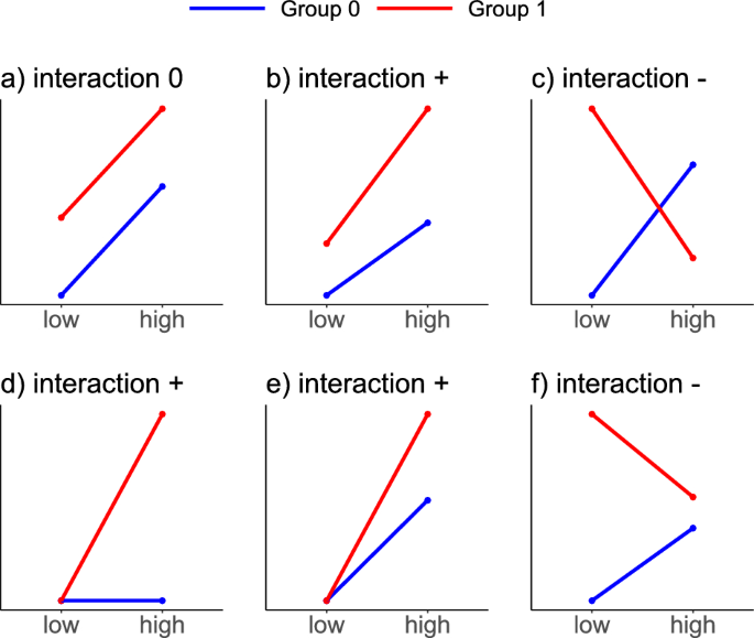
Schematic depiction of data scenarios without and with IE. (a) Group 0 (blue) and 1 (red) both have a positive effect for treatment high compared to low and a positive group effect, but no IE. (b) As in (a), but with an additional positive IE. (c) Negative IE between group and treatment. (d) No treatment effect for group 0. The treatment effect for group 1 is entirely represented by the IE. (e) Both groups display a positive treatment effect and there is no group effect in the treatment category low, only in high, i.e. an IE is present. (f) Negative IE between group and treatment, but no line crossing as in (c).
When two or more factors are of interest in an experiment, one should consider including IEs in the statistical model. Only using additive or main effects may not result in adequate modeling of the data. In Fig. 1, different effect scenarios are visualized using interaction plots for the case of two factors of interest, e.g. some group (0 = blue, 1 = red) and a compound with low and high concentration. In Fig. 1a, there is no interaction between the group and the concentration: The increase of the response from the low to the high concentration is the same for group 0 and group 1. At the same time, for a fixed concentration, the difference in the responses between group 0 and group 1 is the same. One can describe the absence of an IE graphically, biologically, and mathematically.
-
Graphically, an additive effect or the lack of an IE results in parallel lines between the two groups.
-
Biologically, the effect of the concentration does not interact with the effect of the group, because it is always the same increase in response from low to high concentration, regardless of the group.
-
Mathematically, considering two factors with two levels each, a classical linear model, or equivalently an ANOVA model, with only additive effects for the two factors and normal noise is appropriate to model the data. This formalizes to
$$begin{aligned} y_j = mu + alpha cdot g_j + beta cdot c_j + varepsilon _j end{aligned}$$
(1)
where j indicates the sample, (g_j) indicates if the jth sample is in group 0 ((g_j = 0)) or in group 1 ((g_j = 1)), and (c_j) indicates if the j-th sample is exposed to the low concentration ((c_j = 0)) or the high concentration ((c_j = 1)).
The mean difference in the responses for group 1 compared to group 0 is (alpha) and for increasing the concentration from low to high, the mean difference is (beta).
For example, if the j-th sample is in group 0 ((g_j = 0)) and exposed to the low concentration ((c_j = 0)), the expected response is (mu + 0 cdot alpha + 0 cdot beta) = (mu). The intercept (mu) represents the mean response in the reference group (0) with the reference concentration (low).
The contrary case, the presence of a clear IE with a changed direction for the concentration effect, is depicted in Figure 1c. The crossing lines mean that the effect of a concentration increase is not additive (it is not the same within both groups). Instead, the concentration effect depends on the group, i.e. there is an interaction with the group effect. For group 0, an increase in the concentration leads to an increase in the response, whereas for group 1, an increase in the concentration leads to a decrease in the response. The additive model (1) can not capture this interaction as the model fit would force parallel lines into the effect plot. Mathematically, a model that accounts for the interaction between group and treatment is, therefore, an extension of the model in Eq. (1) by adding the IE (gamma):
$$begin{aligned} y_j = mu + alpha cdot g_j + beta cdot c_j + gamma cdot g_jcdot c_j + varepsilon _j. end{aligned}$$
(2)
If the j-th sample is exposed to the higher concentration ((c_j=1)) and is in group 1 ((g_j = 1)), then the mean response is (mu + alpha + beta + gamma). The interaction term (gamma cdot g_jcdot c_j) allows the lines in the interaction plot to be non-parallel. It is important to note that an IE does not necessarily visualize as a crossing of lines in an interaction plot, but simply non-parallel lines, such as in the examples shown in Fig. 1b, d, e, and 1f. We elucidate the use of IEs when analyzing real data in the context of biological research questions in “When do interaction effects capture the research question?”.
Interaction effects calculated with DESeq2
In this section, we explain the mathematical background of gene expression modeling with the popular R-package DESeq2 4. Details on statistical concepts presented here may not be relevant to readers who are more application-oriented and can be ignored without risking comprehension of the remaining sections. However, to understand an IE in more depth, we encourage to understand the parameters in the model formula (4).
Consider the count matrix K, where (K_{ij}) are the count reads of gene i for sample j, (i in {1,…,n}), (j in {1,…,m}). To model the count data, DESeq2 uses a generalized linear model with a negative binomial distribution (K_{ij} sim text {NB}(mu _{ij}, tau _i)) with mean (mu _{ij}) and gene-specific dispersion (tau _i).
The mean of the observed counts (mu _{ij} = s_j q_{ij}) is modeled with the parameter (q_{ij}), which is proportional to the expected true concentration of fragments for sample j and rescaled with a sample-specific size factor (s_j). The parameter (q_{ij}) is modeled with a generalized linear model using the logarithmic link: (text {log}_2(q_{ij}) = sum _r beta _{ir} x_{jr}). In a factorial design, (x_{jr} in {0,1}) indicates if the rth explanatory variable applies to sample j, such that for the ith gene, (beta _{ir}) is the (log _2)FC for factor level r compared to the reference factor level.
For our application example (“Data” ), the model has one factor for the diet (two values) and one factor for the week (six values). A model with the parameters for the week and diet without interaction is fitted for each gene i, (1 le i le 35,727). In the following, we suppress the gene index i and consider the sample (mouse) index j. The model used in DEseq2 is then
$$begin{aligned} text {log}_2(q_{j}) = mu + alpha cdot d_{j} + sum _{r = 2}^6 beta _{r}cdot w_{jr}, end{aligned}$$
(3)
where (mu) (intercept) denotes the response at the reference (SD and week 3), and (alpha) is the WD (main) effect. The variable (d_{j}) is binary with value 0 for the SD and value 1 for the WD. The parameters (beta _r), (rin {2,…,6}), correspond to the week effects. The variable (w_{jr}) is the indicator variable for the week, i.e. (w_{j2}=1) only for week 6.
Now, adding an IE, the model is
$$begin{aligned} text {log}_2(q_{j}) = mu + alpha cdot d_{j} + sum _{r = 2}^6 beta _{r}cdot w_{jr} + sum _{r = 2}^6 gamma _{r}cdot d_{j}cdot w_{jr}. end{aligned}$$
(4)
The parameter (gamma _{2}) denotes the IE between the factor diet and the factor week, comparing week 6 to week 3. The parameter (gamma _{3}) refers to the interaction between the diet and week, comparing week 30 to week 3, and so on. Due to the (log _2) transformation for the sample concentration (q_j), the parameters must all be interpreted accordingly. For example, an IE of (gamma _2=3) means that the difference between the diet effect in week 3 and the diet effect in week 6 is (2^3=8), or has a FC of 8.
When do interaction effects capture the research question?
In RNA-Seq experiments, often the case of two factors, e.g. treatment and genotype, are analyzed, and it is of interest whether the effect of the treatment differs between the genotypes (in certain genes). The research question might be formulated as: Does the genotype affect the treatment effect? IEs capture such a research question and they should therefore be considered for the analysis.
In our application example, the two factors are diet and week, where diet is either a WD or a SD and week indicates the feeding duration. In this dataset measurements for different time points are available, and we focus on the two shortest durations, 3 weeks and 6 weeks, to explain the IE concept. The 3-week time point can be considered the reference level of the factor week. The research goal is to identify genes where activation/deactivation from weeks 3 to 6 induced by the WD is different compared to the SD. Mathematically, this research question translates into identifying genes with an IE between diet and week. Consequently, the use of a model that includes an IE should be considered.
How do interaction effects capture the research question?
To explain how IEs capture the research question, we visualize the benefit of adding IEs to a linear model, using our example dataset. In Fig. 2, for the mice groups, for each combination of diet type and week, expression values and fitted means are plotted, exemplary for one selected gene. Once no IEs are included in the model (Fig. 2, left), and once IEs are included (Fig. 2, right).
Without IEs, the estimated effect differences between the diets, represented by arrows, are mathematically forced to be the same across all weeks (vertical lines have the same length).
Consequently, in week 3, the effect is markedly overestimated, as the arrow between SD and WD is larger than the pure difference in group means. In contrast, if an IE is used (Fig. 2, right), then the group means estimated by the model capture well that the diet effect varies across weeks. The mathematical formulas of the estimated effects represented by the arrows are explained in “Interaction effects calculated with DESeq2”.
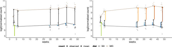
Visualization of the fitted model without IE (left) and with IE (right) for the mice dataset, for the gene identifier ENSMUSG00000069170 (Adgrv1). The arrows represent the estimated (log _2)FCs according to Eq. (3) for the left fit, and Eq. (4) for the right fit. For both fits, (mu) (green arrow) is the expected mean gene expression level for the reference values three weeks and SD, and (alpha) (vertical dark grey arrows) is the estimated FC between SD and WD at each week. Further, both models include the week effects (beta _r) (blue arrows). The right model additionally includes interaction effects (yellow, orange, and red arrows) that correspond to (gamma _r) in formula (4).
Comparison of methods for estimating interaction effects
In this section, we compare the results obtained by fitting an interaction model between two factors (called Method II in the following) with a far more popular alternative, which we call Method I. The alternative approach avoids the direct modeling of an IE between two factors as follows: The data are split with respect to the second factor (e.g. week) into two groups (G_0) and (G_1). Then for group (G_0) and (G_1) separately, a model comparing the groups with respect to the first factor (e.g. diet) is fitted. Finally, it is analyzed, if for one group, typically the reference group (G_0), no significant effect is observed, and for the other group (G_1), there is a significant effect present.
The differences between the two approaches are illustrated and discussed on the mouse dataset, where for Method I the groups (G_0) and (G_1) are defined by week 3 (as reference) and week 6 (or larger week numbers, respectively). The models per week contain only one factor (diet) with two levels, SD and WD. Since separate models are fitted per week, the model-wise diet effect is allowed to vary across weeks.
When interpreting the results of the differential expression analysis, a consideration of both statistical significance and biological relevance is necessary: A p-value smaller than the significance level, which constitutes a statistically significant result, does not necessarily mean that the mean effect level, given here by the (log _2)-Fold Change ((log _2)FC), is of relevant size. On the other hand, a mean effect level larger than a pre-specified threshold, motivated by the biological context, does not always correspond to small p-values 11. Thus, to interpret a gene to be a differentially expressed gene (DEG), we always require two conditions to be fulfilled: The (FDR-adjusted) p-value is smaller than a significance level, and the (log _2)FC is larger than a pre-specified threshold.
For the mouse dataset and the separate models (Method I), only those genes that show a diet effect (both significant and relevant) in week 6, but not in the reference week 3, are considered DEGs. The motivation is that interesting genes show no effect at the reference time point, where the diet had too little time to cause a differential effect, but later (at 6 weeks) the diet causes such a difference. For the interaction model (Method II), not two models but only a single model is fitted. To detect DEGs, one simply checks if the estimated IE is both significant and relevant.
-
Method I (Separate): Separately for each week: Fit a one-factor model (two-group comparison, see equation (1)).
A gene is DEG if the diet effect is both significant and relevant in week 6, but not both in week 3.
-
Method II (Interaction): Fit a two-factor model between week and diet (including week, diet, and interaction), see equation (2).
A gene is DEG if the IE is both significant and relevant.
To visualize the differences between the decision outcomes (gene is DEG or not) of Method I and II, Fig. 3 displays 7 cases using simulated data scenarios. The data are generated with constant residual variance, so that the decision is not influenced by differing variance values, but only by the estimated effect (arrow lengths).
-
Case 1: Within both weeks, the estimated diet effect is not relevant (dotted green effect arrow). There is hence is no DEG by Method I. Since the effects are of similar size, the IE estimated by Method II (pink arrow) is not significant, and neither Method II classifies the gene as DEG.
-
Case 2: In week 3, the effect is not relevant, in week 6 it is both significant and relevant. This leads to a significant IE for Method II. Therefore, both Method I and Method II classify the gene as DEG.
-
Case 3: The diet effect is significant in both weeks. Since it is significant in week 3, Method I does not classify the gene as DEG. However, the diet effect in the second week is much larger, such that the IE is significant, and Method II classifies the gene as DEG.
-
Case 4: Similar to case 3, but the effect direction of the diet effect changes: In the first week, there is a positive effect, and in the second week a negative effect. Again, only Method II classifies the gene as DEG.
-
Case 5: In week 3, the diet effect is just below the significance level, whereas in week 6 it is just above the significance level. Therefore, Method I labels the gene as DEG. For Method II, the IE is not significant as the diet effect does not differ much between the weeks. Method II does not label the gene as DEG.
-
Case 6: Similar to case 4, but the effect in week 3 is not significant. Now both methods classify the gene as DEG.
-
Case 7: The direction of the diet effect changes. It is positive in week 3 and negative in week 6. Within each week, the effect size is not significant, therefore Method I classifies the gene as not DEG. The overall change in the effect represented by the IE is significant. Therefore, Method II labels this gene as DEG.
Implementation
For all calculations, R12, version 4.2.2, and the packages DESeq24, version 1.38.1, and topGO13, version 2.50.0, were used for determining DEGs and performing gene ontology enrichment analyses (GO EA), respectively. The entire code is shared on GitHub (https://github.com/jcduda/gene_expression_interaction). We specify the models of Method I and II in DESeq2 using
-
Method I: DESeqDataSet(gse, design = (sim) diet)
-
Method II: DESeqDataSet(gse, design = (sim) diet + weeks + diet:weeks)
In the example, the code for Method I is applied twice for separate weeks, i.e. for two different data sets ‘gse’, while the code for Method II is applied only once. Note that a model based on (sim) diet + weeks results in the same parameter values for each week, making it unsuitable for comparison with Method I and Method II, see Fig. 2.
One notable preprocessing step was the filtering. Removing only genes with less than ten counts over all samples resulted in a peak of the estimated diet effect at 0.206 (Supplementary Fig. 1). However, removing genes with more than 50% of samples with 0 counts leads to reasonably estimated effects without artifactual spikes in the histogram (Supplementary Fig. 2). Further, we shrunk the estimated effects using approximate posterior estimation with the lfcShrink function14. Effects that are non-zero only due to noise are shrunk to zero, while large, reliable effects are not affected.
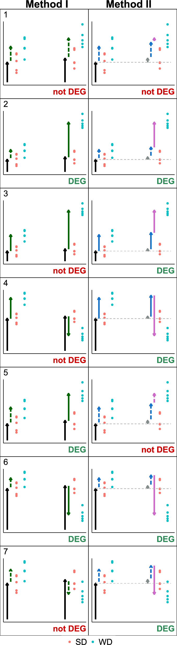
Visualization of seven example scenarios with different main effects and IEs, leading to different decisions for Method I (left column) and Method II (right column). Dots represent data points (blue: SD, red: WD; left: 3 weeks, right: 6 weeks), arrows represent effects (black: reference mean, green: main effect of diet, purple: IE). Dotted arrows indicate non-relevance (absolute effect size below threshold), solid arrows represent relevant effects. Dotted arrows are only shown for the main effects of IEs. The label ’DEG’ below a scenario indicates if the respective method classifies a gene as DEG (green) or not DEG (red).
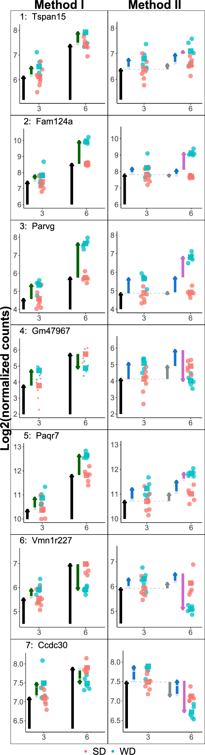
Example genes that are, according to DEG decision cases 1–7, not always classified in the same way by Method I (left) and II (right). Note that the original data are the same per gene (row), but due to the differences between Method I and II, background normalizations yield slightly different data for each gene. For normalization, DESeq estimates the library sizes as the median of the ratios of observed counts9. See caption of Figure 3 for an explanation of the arrows.
- SEO Powered Content & PR Distribution. Get Amplified Today.
- PlatoData.Network Vertical Generative Ai. Empower Yourself. Access Here.
- PlatoAiStream. Web3 Intelligence. Knowledge Amplified. Access Here.
- PlatoESG. Carbon, CleanTech, Energy, Environment, Solar, Waste Management. Access Here.
- PlatoHealth. Biotech and Clinical Trials Intelligence. Access Here.
- Source: https://www.nature.com/articles/s41598-023-47057-0