Stem Cell

An AI-based segmentation and analysis pipeline for high-field MR monitoring of cerebral organoids – Scientific Reports

Time Stamp: November 30, 2023 7:00 PM
Source Node: 363796

The code to reproduce the results is publicly available on GitHub (https://github.com/deiluca/cerebral_organoid_quant_mri). All MRI images and annotations for organoid segmentation, global cysticity classification, and local cyst segmentation generated for this work are publicly available on Zenodo (https://zenodo.org/record/7805426).

Differentiation of cerebral organoids

Organoids were generated according to²⁶ with minor modifications. Wildtype iPSCs were singled and seeded at a density of 8 × 10⁴ cells/ml in a V-shaped 96 well plate in organoid formation medium (DMEM/F12, KnockOut Serum Replacement, NEAA, ß-mercaptoethanol) supplemented with 4 ng/ml bFGF (Peprotech) and Y-27632 (50 µM; StemCell Technologies) to induce embryoid body (EB) formation. The following day, the medium was exchanged to remove Y-27632 and lower the bFGF concentration to 2 ng/ml. On day 5, neural induction was initiated by exchanging the medium to neural induction medium (DMEM/F12, N2 supplement, NEAA, glutamine (all ThermoFisher), 1 µg/ml heparin (Sigma)) with a medium change on day 7. On day 9, EBs were embedded into Matrigel (Corning; growth factor reduced) droplets and cultivated until day 13 in organoid differentiation medium (ODM) 1 (DMEM/F12:Neurobasal medium 50:50, NEAA, glutamine, penicillin/streptomycin, N2 supplement, B27 supplement w/o vitamin A (all ThermoFisher), insulin (Sigma), ß-mercaptoethanol (ThermoFisher)). On day 13, organoids were excised from the droplets and transferred into a 12-well plate containing organoid differentiation medium 2 (DMEM/F12:Neurobasal medium 50:50, NEAA, glutamine, penicillin/streptomycin, N2 supplement, B27 supplement with vitamin A, insulin, ß-mercaptoethanol) and placed on a shaker in the incubator with medium exchange every 2–3 days. After imaging, the organoids were transferred back to the plate containing fresh medium and placed on the orbital shaker (Sunlab, 55 rounds/minute) for further development.

Brightfield imaging

Brightfield images were taken using a Leica DMi1 microscope with included camera using LAS EZ software (Leica). Images were taken with a 10 × magnification from day 1 until day 9 of differentiation and were further followed with a 5 × magnification from day 12 until day 29.

MRI

For MR measurements, organoids were transferred to 1.5 ml Eppendorf tubes containing standard ODM (T2-time of ~ 64 ms in this experimental setting) and conveyed to the MRI using warming packs for temperature control. In total, nine organoids were scanned at varying time points over a period of 64 days, resulting in 45 individual samples. Three Eppendorf tubes were placed next to each other in a holder, thus allowing simultaneous imaging of three organoids (Supplementary Fig. 6). Nine control organoids not undergoing MRI served as handling control. Before and after imaging, the medium was analyzed in both groups using a blood gas analyzer which showed that MRI had no specific negative effect on organoid health (Supplementary Table 3).

MRI was performed at room temperature using a high-field 9.4 Tesla horizontal bore small animal experimental NMR scanner (BioSpec 94/20 USR, Bruker BioSpin GmbH, Ettlingen, Germany) equipped with a four-channel phased-array surface receiver coil. Compared to common field MRI field strengths ranging from 1 to 7 Tesla, high-field 9.4 Tesla offers significantly improved spatial resolution and enhanced signal-to-noise ratio²⁷. The MR protocol included the following sequences:

1.

High-resolution T2*-weighted gradient echo sequence: 3D sequence, echo time (TE): 18 ms, repetition time (TR): 50 ms, 80 µm isotropic resolution, acquisition matrix: 400 × 188 × 100, flip angle: 12˚, number of averages: 1, duration: 15 min 40 s. This sequence was chosen to allow for accurate isotropic imaging and to account for potential susceptibility effects caused by e.g. neuromelanin²⁸, cellular debris or calcifications.
2.

DTI-spin echo sequence: 2D sequence, TE: 18.1 ms, TR: 1200 ms, 100 µm in-plane resolution, acquisition matrix: 120 × 50, slice thickness: 1.5 mm, number of diffusion gradient directions: 18 + 5 A0 images, b-values: 0/650 s/mm², gradient duration: 2.5 ms, gradient separation: 15.5 ms, flip angle: 130°, number of averages: 1, duration: 23 min 05 s. This sequence was included to account for organoid inner structure including nerve fiber growth²⁹.

Organoid segmentation

Organoid segmentation was performed to assign each image voxel to one of two categories: organoid or non-organoid.

For MRI, we used min–max normalized images from the T2*-w sequence. Since simpler methods like Multi-Otsu’s threshold³⁰ and a 2D U-Net³¹ did not deliver convincing results (Supplementary Table 2), we used a 3D U-Net³² for efficient (Supplementary Table 4) organoid segmentation. We trained the model with Adam (learning rate 1 × 10⁻³, weight decay 1 × 10⁻⁷) for 2000 iterations with batch size 1 and a weighted combination of binary cross entropy and Dice loss (1:10).

For brightfield imaging, Otsu’s threshold³³ did not yield compelling results as well (Supplementary Table 5). Therefore, we used the SegFormer model³⁴, implemented in³⁵, for state-of-the-art 2D segmentation. We trained the model with Adam (learning rate 1 × 10⁻⁴, weight decay 1 × 10⁻¹) for 2000 iterations with batch size 1 and a weighted combination of binary cross entropy and Dice loss (1:10). The config files for SegFormer training are provided on GitHub.

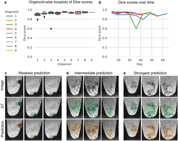
For evaluation of both models, we used the Dice score, which is commonly used to quantify the performance of image segmentation methods. It is defined as two times the area of the intersection divided by the total number of voxels in the ground truth and predicted segmentation (Eq. 1). A perfect segmentation corresponds to a Dice score of 1.

$$Dice, score=frac{2cdot |Acap B|}{|A|+|B|}$$

(1)

To get an unbiased estimate of the models’ performance, we used organoid-wise Leave-One-Out Cross-Validation (LOOCV). For each of the nine LOOCV splits, all images of one organoid are used for model testing, the remaining images of all other organoids are used for model training and model validation. For each LOOCV split, we used a random 80% training, 20% validation split for model selection. The Dice score in the Results section refers to the model performance on the LOOCV test set.

Global cysticity classification

Global cysticity classification aims at determining the overall organoid cysticity: cystic (low-quality) or non-cystic (high-quality). To provide a reference ground truth based on the T2*-w sequence, an organoid was categorized as cystic if a cystic structure was detected within the organoid, corresponding to standard quality assessment on brightfield imaging (Supplementary Fig. 3) as previously reported^8,9. Otherwise, it was categorized as non-cystic.

For automatic classification in MRI, we constructed the simple metric compactness which serves as an environment-based estimator of organoid cysticity (Eq. 2). It is based on the idea that cysts are filled with similar fluid like the medium under the assumption of relative B1-homogeneity in a stereotyped region close to the surface coil. Therefore, the more similar the organoid intensities are to the medium intensities, the more cystic the organoid is.

$$begin{aligned}&Compactness: = absleft[ {upmu left( {int_{{org}} } right) – upmu left( {int_{{medium}} } right)} right] hfill &mu left( X right): = frac{1}{{left| X right|}}sum _{{x in X}} x hfill &abs(x) = left{ {begin{array}{ll} {x;,if;x > 0} { – x;,otherwise} end{array} } right. hfill &{text{A}}{ setminus }{text{B}} = { {text{x}} in {text{A}}:{text{x}} notin {text{B}}} hfill &int_{{org}} = { {text{intensities}};{text{of}};{text{organoid}};{text{voxels}}} hfill &int_{{medium}} = { {text{intensities}};{text{of}};{text{medium}};{text{voxels}}} setminus int_{{org}} hfill end{aligned}$$

(2)

While int_org was derived from the ground truth organoid segmentations, int_medium was determined by applying Otsu’s threshold³³ 2D-wise along all organoid-containing coronal planes (Supplementary Fig. 7). The first and last organoid-containing coronal planes were discarded to filter artifacts caused by noisy medium intensities.

For brightfield imaging, concepts like compactness are not applicable due to heterogeneous microscopy backgrounds and the limited spatial visibility of cysts in the 2D image (Supplementary Fig. 3). Therefore, we used the state-of-the-art neural network ResNet34³⁶ for binary classification, implemented in³⁷. The model was trained with Adam (learning rate 1 × 10⁻⁶, weight decay 0) for 30 epochs with batch size 16 and a binary cross entropy loss. On-the-fly image augmentations included random rotation (0–360 degrees), random resized crop (scale 0.3–1.0, ratio 1.0) and ColorJitter (brightness = 0.1, saturation = 0.1, contrast = 0.1) to account for large variations in organoid size and color.

For the evaluation of compactness and the ResNet34, we used the area under the Receiver Operator Characteristic curve (ROC AUC). ROC AUC is a common metric for the evaluation of binary classification problems; a perfect classifier achieves a ROC AUC of 1. Since in contrast to compactness, the ResNet34 requires training, we used organoid-wise LOOCV for model evaluation.

To further probe tissue characteristics of cystic and non-cystic organoids, parameter maps (Trace; FA; 1st, 2nd_, and 3rd Eigenvalues) were extracted from the DTI sequence using the built-in analysis tool (Paravision 6.0, Bruker BioSpin GmbH, Ettlingen, Germany). We used a two-sided T-test to test for significantly different average diffusion and used Holm-Šídák to adjust for multiple testing.

Local cyst segmentation

Local cyst segmentation aims at localizing cysts. For this task, we used the T2*-w sequence and manually annotated cysts. Due to the low-resolution images, especially smaller cysts are difficult to annotate. Therefore, we excluded organoids with less than 1000 voxels (0.51 mm³) in cysts and included 34 samples in total.

For segmentation, we trained and evaluated a 3D U-Net³² as for organoid segmentation but with 5000 training iterations. Local cyst segmentation was performed for MRI images only, because the annotation of cysts in brightfield images was not feasible due the limited spatial visibility of cysts in the 2D images (Supplementary Fig. 3).